Introduction
This is the last post in the series Elegant Data Visualization with ggplot2. In the previous post, we learnt to combine multiple plots. In this post, we will learn to modify the appearance of all non data components of the plot such as:
- axis
- legend
- panel
- plot area
- background
- margin
- facets
Libraries, Code & Data
We will use the following libraries in this post:
All the data sets used in this post can be found here and code can be downloaded from here.
Basic Plot
We will continue with the scatter plot examining the relationship between displacement and miles per gallon from the the mtcars data set.
p <- ggplot(mtcars) +
  geom_point(aes(disp, mpg))
p
Axis
Text
The axis.title.x argument can be used to modify the appearance of the X
axis. In the below example, we modify the color and size of the title using
the element_text() function. Remember, whenever you are trying to modify the
appearance of a theme element which is a text, you must use element_text().
You can use axis.title.y to modify the Y axis title and to modify the
title of both the axis together, use axis.title.
p + theme(axis.title.x = element_text(color = "red", size = 10, face = "italic"))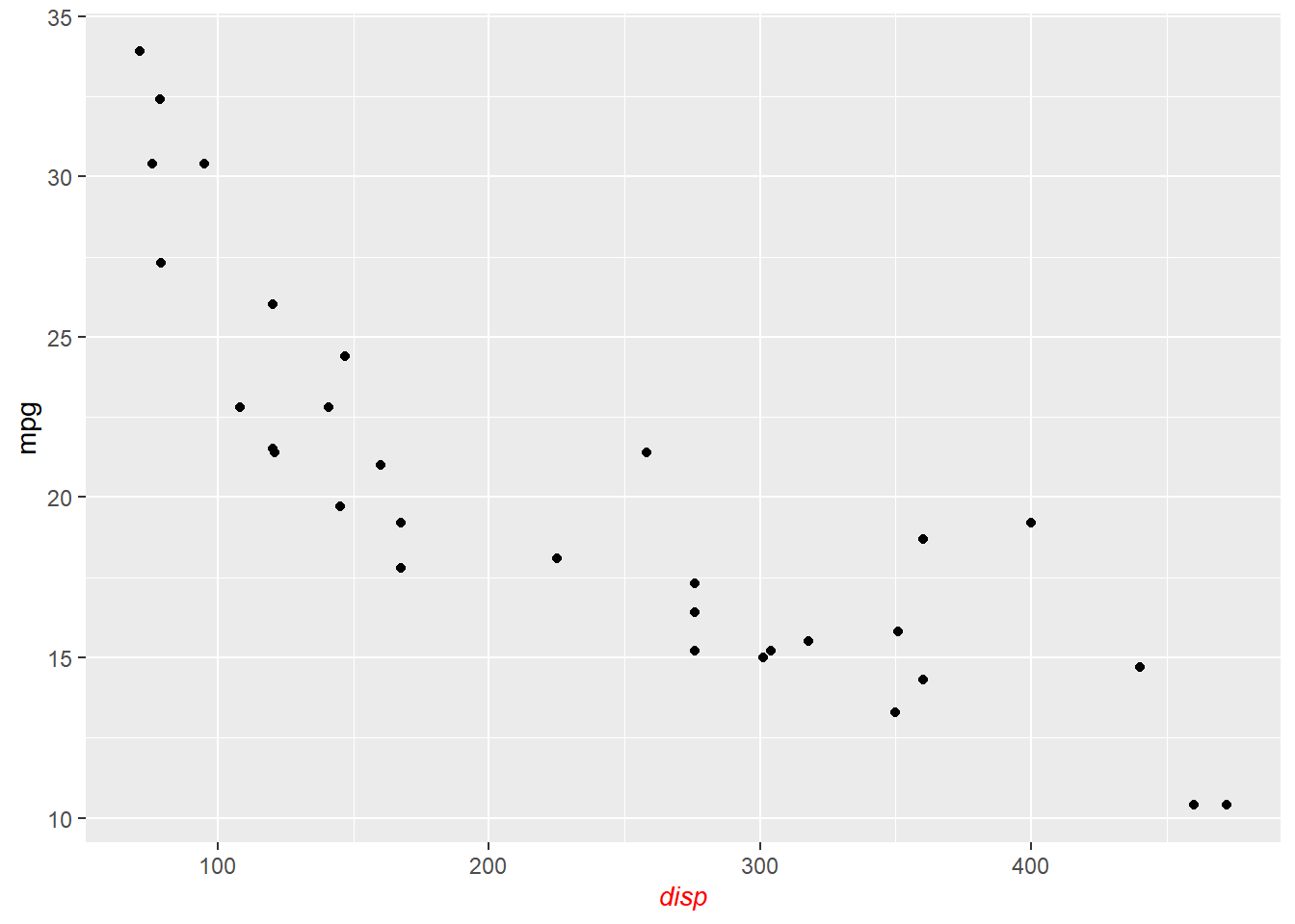
Ticks
To modify the appearance of the axis ticks, use the axis.ticks argument. You can
change the color, size, linetype and length of the ticks using the element_line()
function as shown below.
p + theme(axis.ticks = element_line(color = 'blue', size = 1.25, linetype = 2),
          axis.ticks.length = unit(1, "cm"))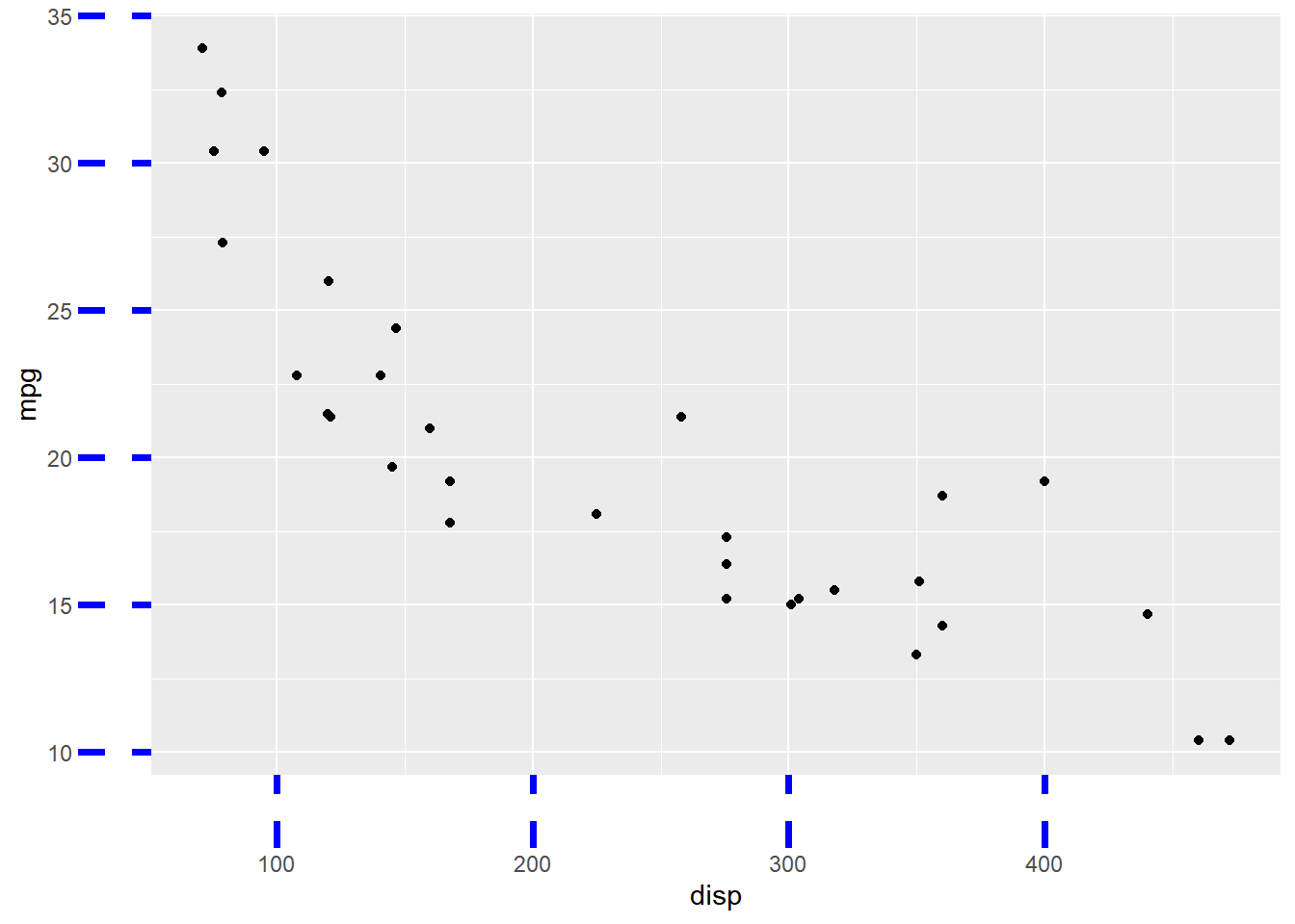
Line
The axis.line argument should be used to modify the appearance of the
axis lines. You can change the color, size and linetype of the line using
the element_line() function.
p + theme(axis.line = element_line(color = 'red', size = 1.5, linetype = 3))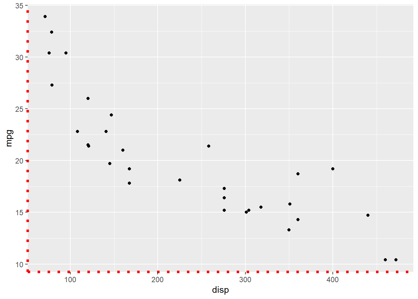
Legend
Now, let us look at modifying the non-data components of a legend.
p <- ggplot(mtcars) +
  geom_point(aes(disp, mpg, color = factor(cyl), shape = factor(gear)))
p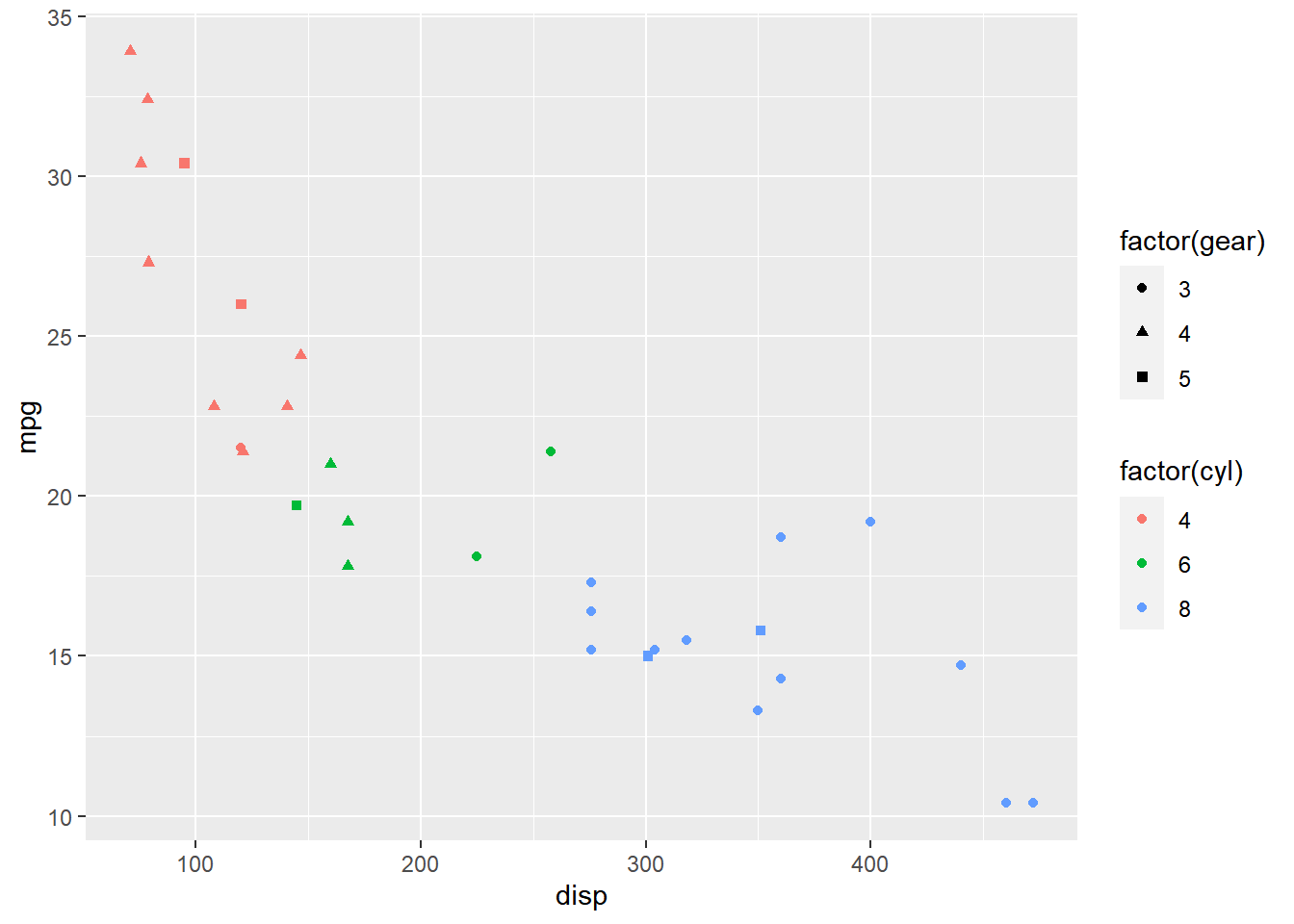
Background
The background of the legend can be modified using the legend.background
argument. You can change the background color, the border color and line type
using element_rect().
p + theme(legend.background = element_rect(fill = 'gray', linetype = 3,
          color = "black"))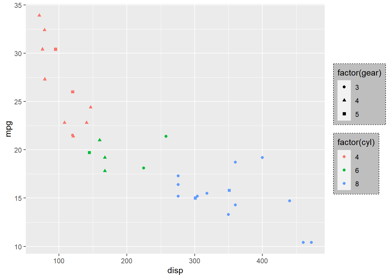
Text
The appearance of the text can be modified using the legend.text argument.
You can change the color, size and font using the element_text() function.
p + theme(legend.text = element_text(color = 'green', face = 'italic'))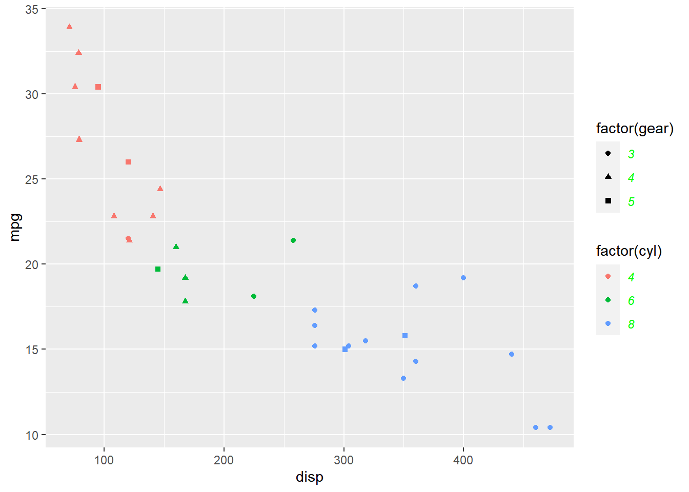
Title
The appearance fo the title of the legend can be modified using the
legend.title argument. You can change the color, size, font and alignment
using element_text().
p + theme(legend.title = element_text(color = 'blue', face = 'bold'),
          legend.title.align = 0.1)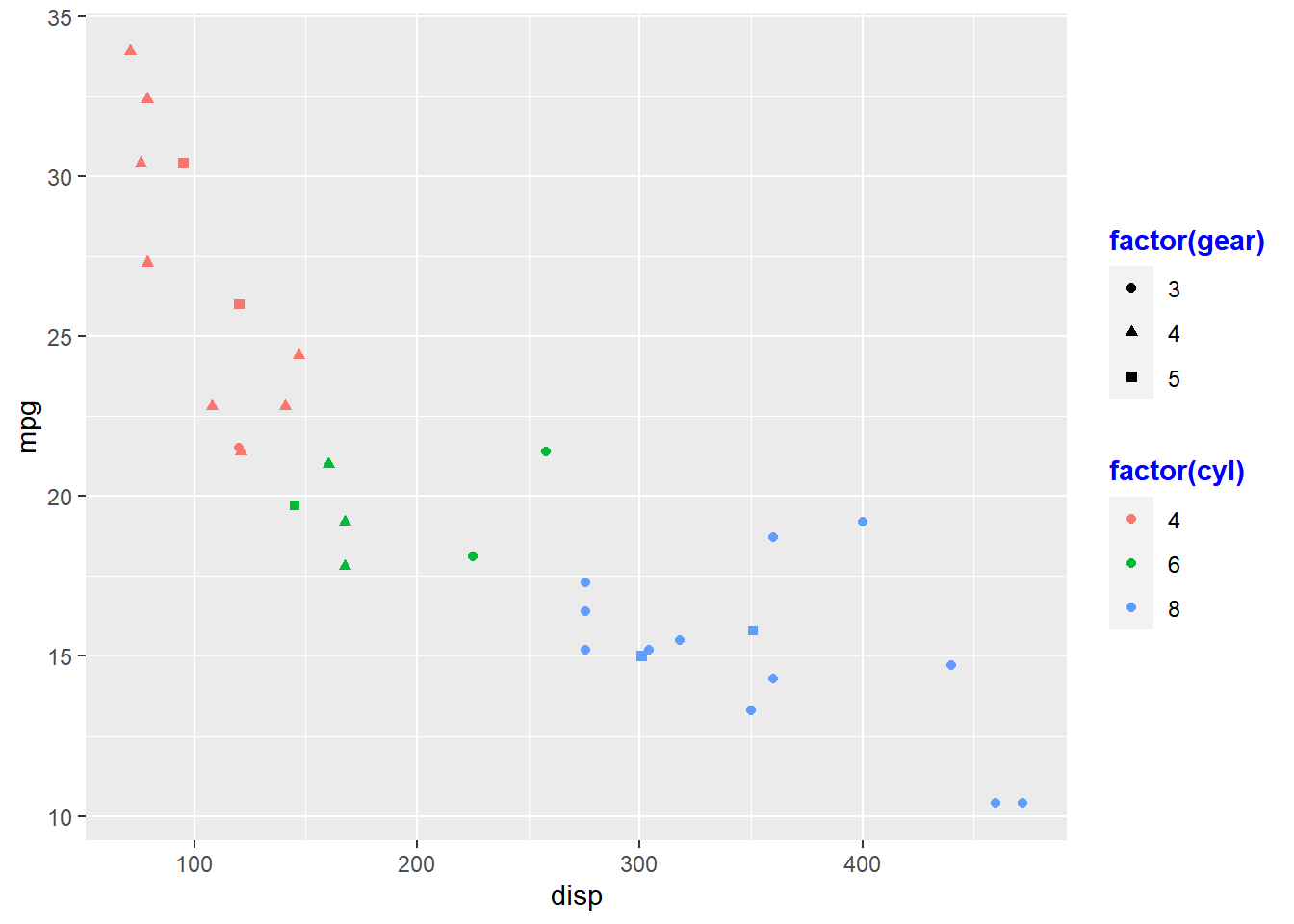
Position
The position and direction of the legend can be changed using:
legend.position- and
legend.direction
p + theme(legend.position = "top", legend.direction = "horizontal")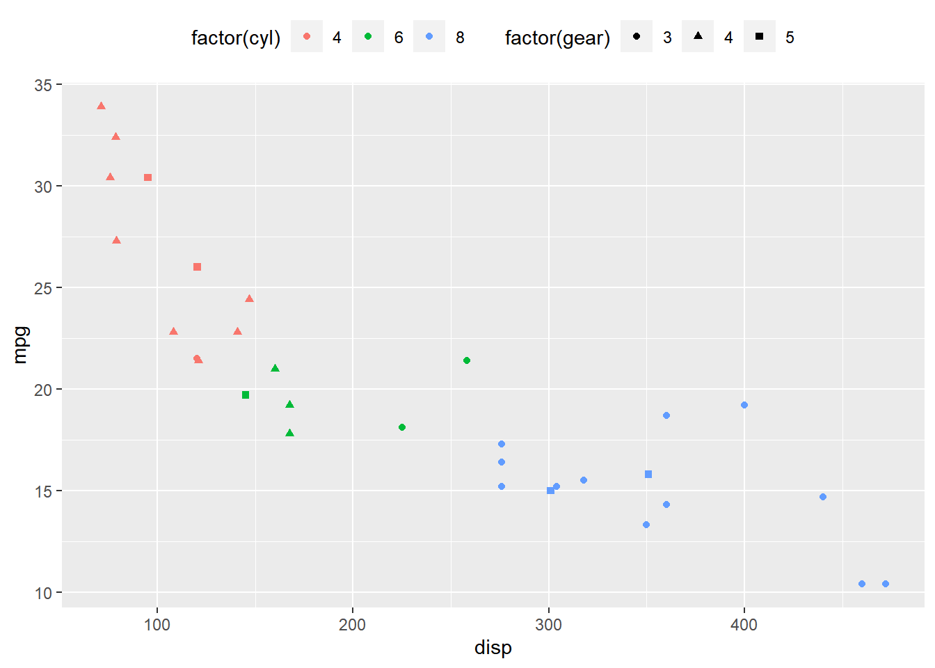
Themes
Classic Dark on Light
ggplot(mtcars) +
  geom_point(aes(disp, mpg)) +
  theme_bw()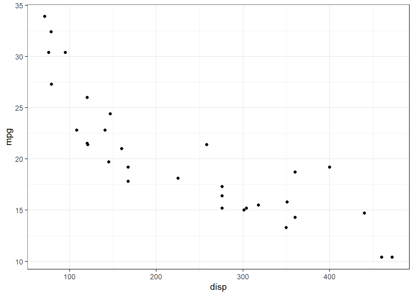
Default Gray
ggplot(mtcars) +
  geom_point(aes(disp, mpg)) +
  theme_gray()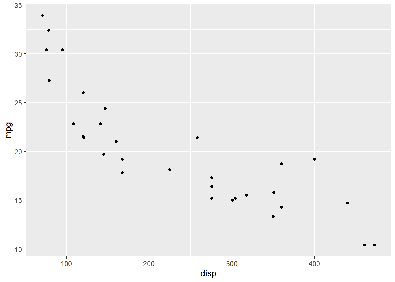
Light
ggplot(mtcars) +
  geom_point(aes(disp, mpg)) +
  theme_light()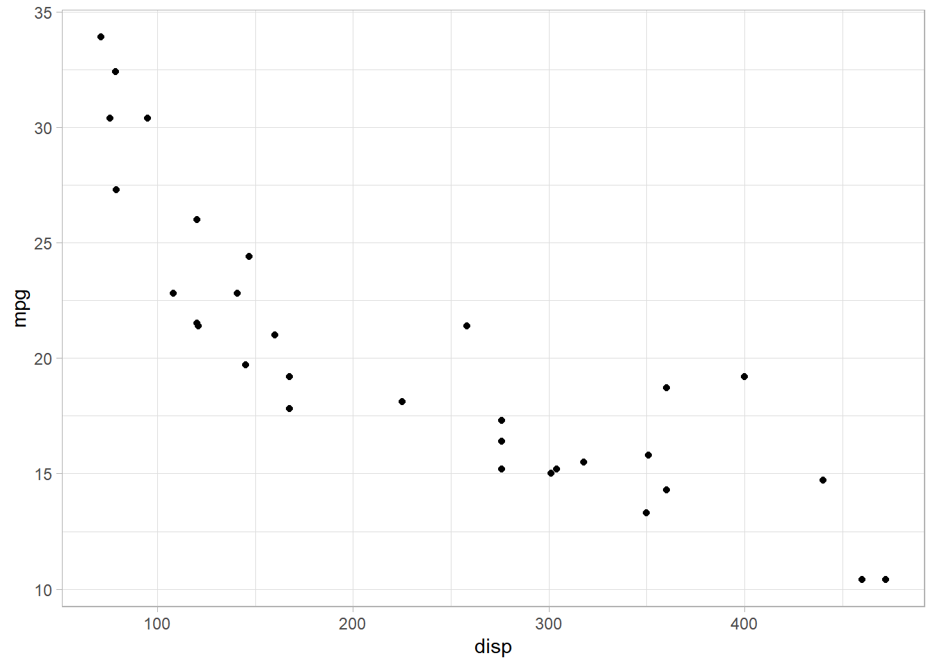
Minimal
ggplot(mtcars) +
  geom_point(aes(disp, mpg)) +
  theme_minimal()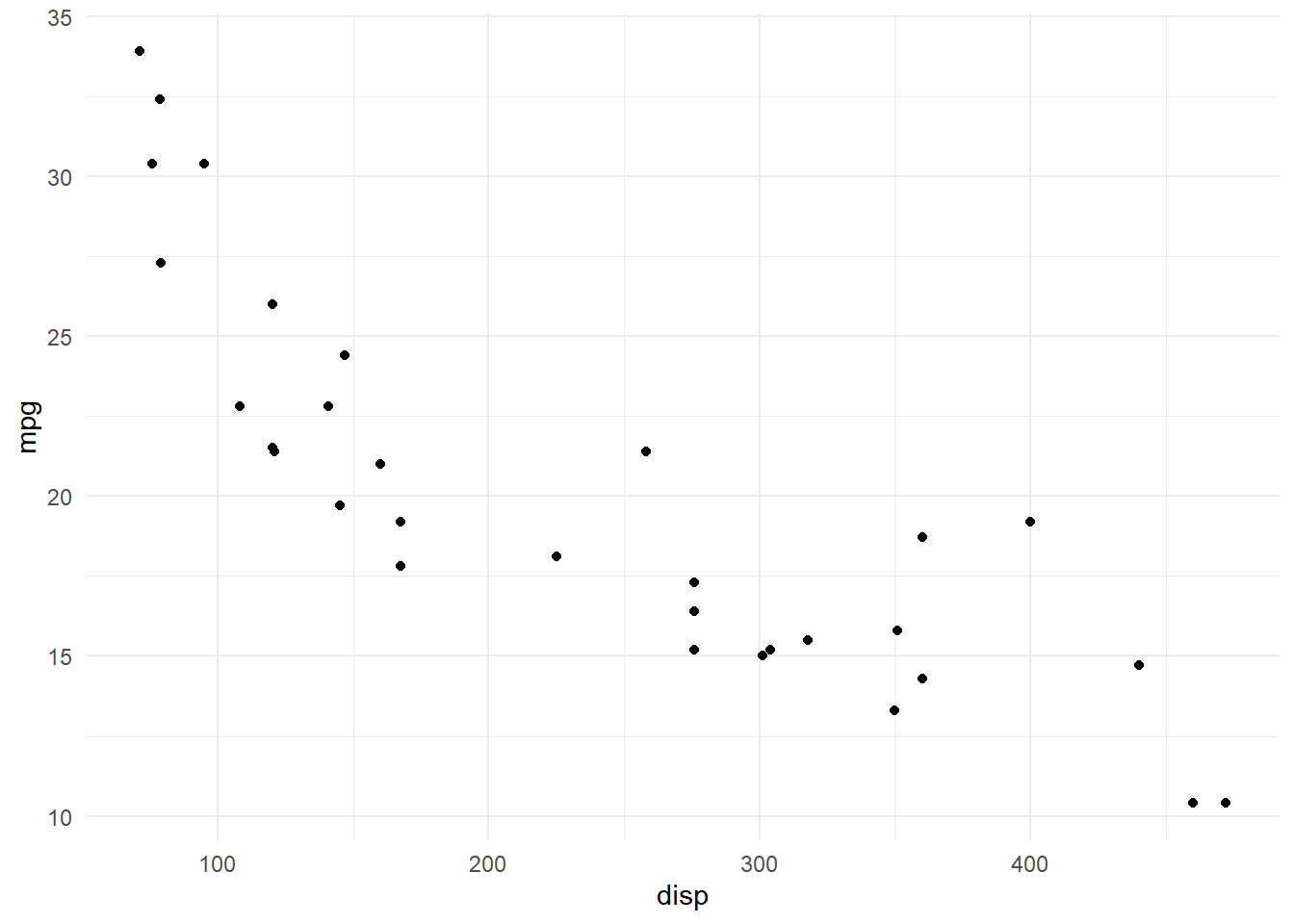
Dark
ggplot(mtcars) +
  geom_point(aes(disp, mpg)) +
  theme_dark()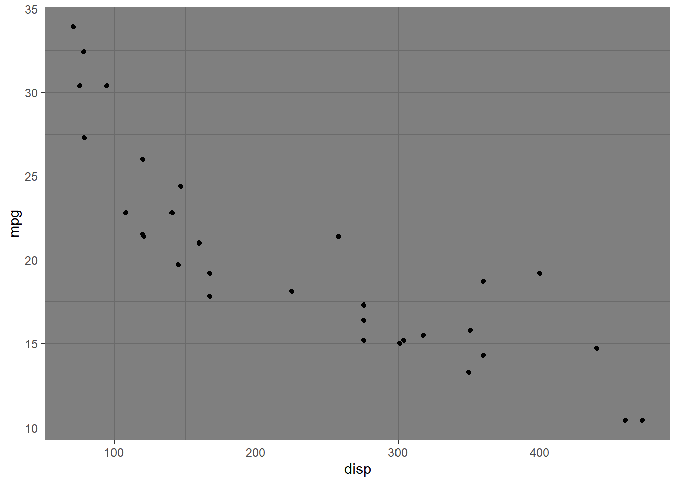
Classic
ggplot(mtcars) +
  geom_point(aes(disp, mpg)) +
  theme_classic()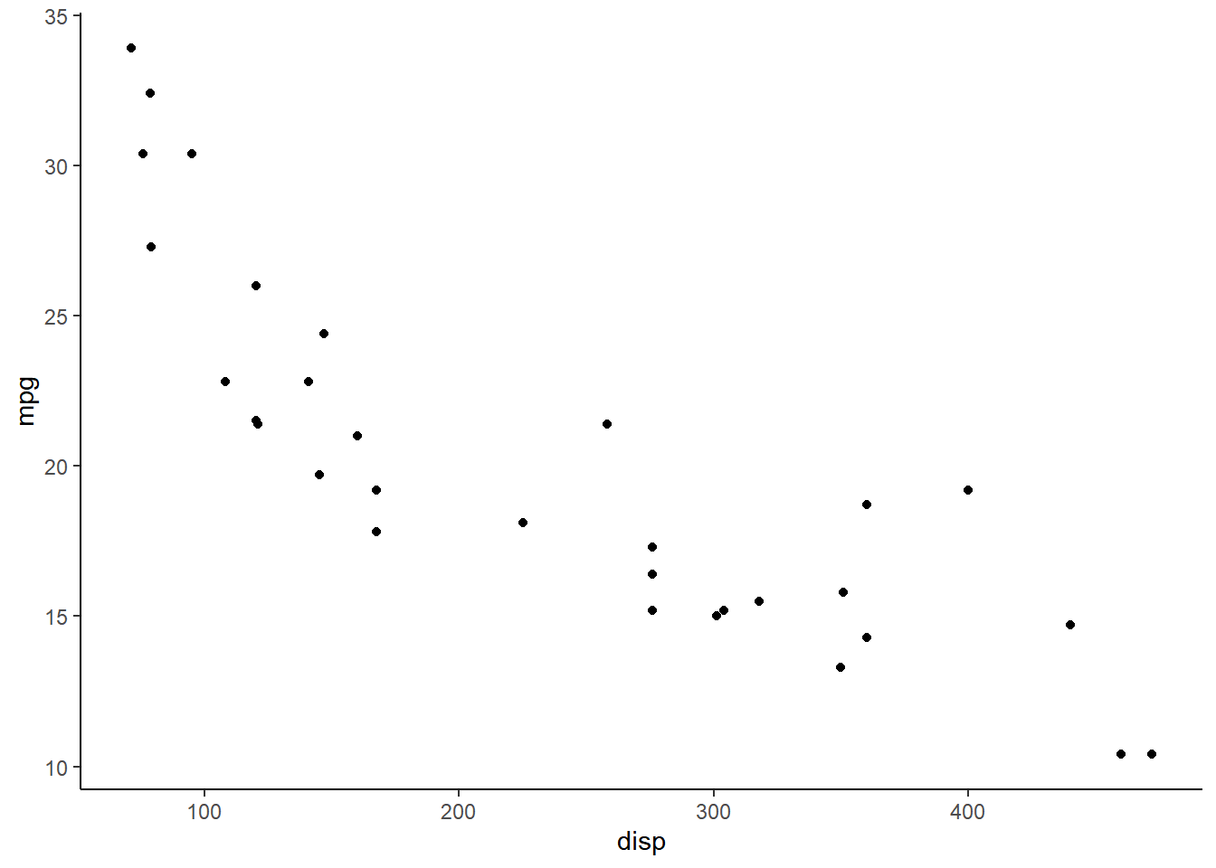
Void (Empty)
ggplot(mtcars) +
  geom_point(aes(disp, mpg)) +
  theme_void()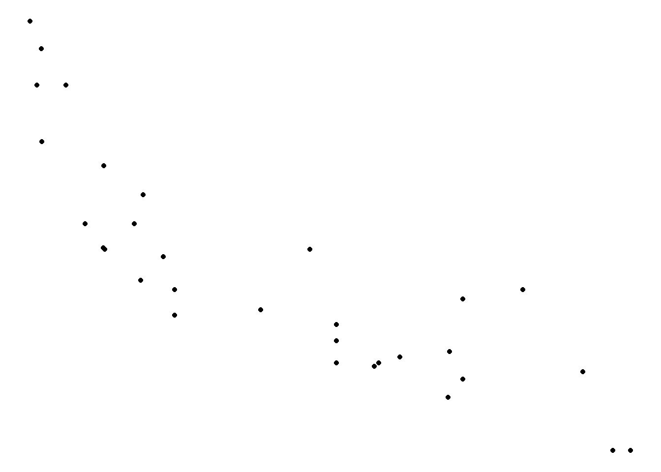
Summary
In this post, we learnt to modify the appearance of all non data components of a plot and about the different themes available in ggplot2. This brings us to the end of the series Elegant Data Visualization with ggplot2.