Create Table
To create a new table, use dbWriteTable(). It takes the following 3 arguments:
-
connection name
-
name of the new table
-
data for the new table
Let us first create a new dataset trial_db. It has 2 columns, x and y, and 10 rows of data. Next, we create a new table of the same name in the database. In dbWriteTable(), we specify the following:
-
con: database connection
-
“trial_db”: name of the table in database
-
trial_data: name of the dataset used to create the table in the database
Ensure that the name of the table in the database is always enclosed in single/double quotes.
# sample data
x          <- 1:10
y          <- letters[1:10]
trial_data <- tibble::tibble(x, y)

# write table to database
DBI::dbWriteTable(con, "trial_db", trial_data)
Let us check if the table has been created.
DBI::dbListTables(con)
## [1] "COMPANY" "DEPARTMENT" "ecom" "trade" "trial_db"
DBI::dbExistsTable(con, "trial_db")
## [1] TRUE
Insert Rows
We can insert new rows into existing tables using:
-
dbExecute()
-
dbSendStatement()
Both the function take 2 arguments:
-
connection name
-
sql statement
In the below example, we insert a new row of data into the trial-db table in the database using dbExecute().</p> <pre class="r"><code>DBI::dbExecute(con, "INSERT into trial_db (x, y) VALUES (32, 'c'), (45, 'k'), (61, 'h')" )</code></pre> <pre><code>## [1] 3</code></pre> <p>Let us check if the new row of data has been inserted into the <code>trial_db</code> table by querying data from the same table.</p> <pre class="r"><code>DBI::dbGetQuery(con, "select * from trial_db")</code></pre> <pre><code>## x y ## 1 18 k ## 2 88 l ## 3 96 m ## 4 24 n ## 5 85 o ## 6 62 p ## 7 67 q ## 8 57 r ## 9 98 s ## 10 13 t ## 11 14 e ## 12 57 f ## 13 5 g ## 14 53 h ## 15 72 i ## 16 85 j ## 17 47 k ## 18 45 l ## 19 6 m ## 20 18 n ## 21 32 c ## 22 45 k ## 23 61 h</code></pre> <p>In the next example, we insert another row of data into the <code>trial_db</code> table in the database using <code>dbSendStatement()</code>.</p> <pre class="r"><code>DBI::dbSendStatement(con, "INSERT into trial_db (x, y) VALUES (25, 'm'), (54, 'l'), (16, 'y')" )</code></pre> <pre><code>## <SQLiteResult> ## SQL INSERT into trial_db (x, y) VALUES (25, 'm'), (54, 'l'), (16, 'y') ## ROWS Fetched: 0 [complete] ## Changed: 3</code></pre> <p>Let us check if the new row of data has been inserted into the <code>trial_db</code> table by querying data from the same table.</p> <pre class="r"><code>DBI::dbGetQuery(con, "select * from trial_db")</code></pre> <pre><code>## Warning: Closing open result set, pending rows</code></pre> <pre><code>## x y ## 1 18 k ## 2 88 l ## 3 96 m ## 4 24 n ## 5 85 o ## 6 62 p ## 7 67 q ## 8 57 r ## 9 98 s ## 10 13 t ## 11 14 e ## 12 57 f ## 13 5 g ## 14 53 h ## 15 72 i ## 16 85 j ## 17 47 k ## 18 45 l ## 19 6 m ## 20 18 n ## 21 32 c ## 22 45 k ## 23 61 h ## 24 25 m ## 25 54 l ## 26 16 y</code></pre> </div> <div id="remove-table" class="section level4"> <h4>Remove Table</h4> <p>To delete/remove a table from the database, use <code>dbRemoveTable()</code>.</p> <pre class="r"><code>DBI::dbRemoveTable(con, "trial_db")</code></pre> </div> <div id="your-turn-1" class="section level3"> <h3>Your Turn</h3> <ul> <li>check if <code>mytable</code> exists in the database</li> <li>create new table <code>mytable</code> using the first 3 rows of <code>mtcars</code> data set</li> <li>list all tables to check if the new table has been created</li> <li>overwrite <code>mytable</code> with the first 10 rows of <code>mtcars</code> data set</li> <li>append the 20th row of <code>mtcars</code> data set to <code>mytable</code></li> <li>create a new table using the last 5 rows of <code>mtcars</code> and append it to <code>mytable</code></li> <li>remove <code>mytable</code></li> </ul> </div> </div> <div id="data-type" class="section level2"> <h2>Data Type</h2> <p>We know of the different data types in R such as integer, numeric/double, logical, factor etc. How do databases treat these data types? To know the data type of a particular value in a database, use <code>dbDataType()</code>. The first input is the database driver and the next is the value whose data type we are seeking. In the below example, we look at the data type of 3 different values in SQLite.</p> <pre class="r"><code>DBI::dbDataType(RSQLite::SQLite(), "a")</code></pre> <pre><code>## [1] "TEXT"</code></pre> <pre class="r"><code>DBI::dbDataType(RSQLite::SQLite(), 1:5)</code></pre> <pre><code>## [1] "INTEGER"</code></pre> <pre class="r"><code>DBI::dbDataType(RSQLite::SQLite(), 1.5)</code></pre> <pre><code>## [1] "REAL"</code></pre> </div> <div id="generate-sql-query" class="section level2"> <h2>Generate SQL Query</h2> <p><code>sqlCreateTable()</code> will generate the SQL statement for simple <code>CREATE TABLE</code> operations. In the below example, it generates the SQL statement for creating table <code>new</code> with two fields <code>x</code> and <code>y</code>.</p> <pre class="r"><code>DBI::sqlCreateTable(con, "new", c(x = "integer", y = "text"))</code></pre> <pre><code>## Warning: Do not rely on the default value of the row.names argument for ## sqlCreateTable(), it will change in the future.</code></pre> <pre><code>## <SQL> CREATE TABLEnew( ##xinteger, ##ytext ## )</code></pre> <p><code>sqlAppendTable()</code> will generate the SQL statement for simple <code>INSERT</code> operations. In the below example, it generates the SQL statement for inserting a new row of data into the <code>trial_db</code> table.</p> <pre class="r"><code>trial_new <- data.frame(x = 30, y = 'k') DBI::sqlAppendTable(con, "trial_db", trial_new)</code></pre> <pre><code>## Warning: Do not rely on the default value of the row.names argument for ## sqlAppendTable(), it will change in the future.</code></pre> <pre><code>## <SQL> INSERT INTOtrial_db## (x,y) ## VALUES ## (30, 'k')</code></pre> <hr> <p> <a href="https://www.youtube.com/user/rsquaredin/" target="_blank"><img src="/img/ad_youtube.png" width="100%" alt="youtube ad" style="text-decoration: none;"></a> </p> <hr> </div> <div id="running-sql-scripts" class="section level2"> <h2>Running SQL Scripts</h2> <p>Once you are connected to a database, you may want to run some SQL queries. So far, we have run the SQL queries in R using function from the DBI package. Using RStudio SQL scripts, we can execute plain SQL queries as shown below. In the first line, we specify the database connection <code>-- !preview conn=con</code> followed by SQL queries. The output can be viewed by clicking on the preview button. We have included a sample SQL script (dbi.sql) which you can open and execute in RStudio.</p> <p><img src="/img/dbi_running_sql_scripts.png" width="100%" style="display: block; margin: auto;" /></p> </div> <div id="knitr-sql-engine" class="section level2"> <h2>knitr SQL Engine</h2> <p>In addition to R, the knitr package can execute code chunks in a variety of languages including SQL. In the below image, we show how to execute SQL queries. First, we establish a DBIconnection to a database in a R code chunk which is then used in a SQL chunk via the <code>connection</code> option (<code>connection = con</code>). Check out the <code>dbi.Rmd</code> file in the resources section.</p> <p><img src="/img/dbi_knitr_sql_engine.png" width="100%" style="display: block; margin: auto;" /></p> <div id="your-turn-2" class="section level3"> <h3>Your Turn</h3> <ul> <li>check the data type of <code>"NULL"</code></li> <li>use SQL script to select <code>duration</code>, <code>n_visit</code> from <code>trade</code> table where <code>device</code> has the value <code>tablet</code></li> <li>create a html report for the above sql query using the knitr SQL engine</li> </ul> </div> </div> <div id="data-transformation" class="section level2"> <h2>Data Transformation</h2> <p>In this section, we will learn to query data from a database using dplyr. We will learn to:</p> <ul> <li>reference data</li> <li>query data using dplyr</li> <li>display query</li> <li>collect data</li> <li>simulate</li> </ul> <div id="reference-data" class="section level4"> <h4>Reference Data</h4> <p>The first step is to reference the table in the database using <code>tbl()</code>. Since we want to use the <code>ecom</code> table from the database, we reference it as <code>ecom2</code> using <code>tbl()</code>.</p> <pre class="r"><code>ecom2 <- dplyr::tbl(con, "ecom") ecom2</code></pre> <pre><code>## # Source: table<ecom> [?? x 11] ## # Database: sqlite 3.30.1 [J:\R\Others\blogs\content\post\mydatabase.db] ## id referrer device bouncers n_visit n_pages duration country purchase ## <int> <chr> <chr> <chr> <int> <dbl> <dbl> <chr> <chr> ## 1 1 google laptop true 10 1 693 Czech ~ false ## 2 2 yahoo tablet true 9 1 459 Yemen false ## 3 3 direct laptop true 0 1 996 Brazil false ## 4 4 bing tablet false 3 18 468 China true ## 5 5 yahoo mobile true 9 1 955 Poland false ## 6 6 yahoo laptop false 5 5 135 South ~ false ## 7 7 yahoo mobile true 10 1 75 Bangla~ false ## 8 8 direct mobile true 10 1 908 Indone~ false ## 9 9 bing mobile false 3 19 209 Nether~ false ## 10 10 google mobile true 6 1 208 Czech ~ false ## # ... with more rows, and 2 more variables: order_items <dbl>, ## # order_value <dbl></code></pre> <p>If you look at the output, <code>ecom2</code> displays a tibble but in the second line it also shows the database information as well. Let us now move on and calculate the average time on site by device type.</p> </div> <div id="query-data" class="section level4"> <h4>Query Data</h4> <p>Let us compute the average time on site for different referrer groups when the visitor browses the site using a laptop. Now, instead of using SQL statement to extract the above information, we will use dplyr. This is especially useful if the user is not well versed in SQL. While dplyr can be used to query data, it is still advisable to learn the basics of SQL.</p> <pre class="r"><code>ecom2 %>% dplyr::select(referrer, device, duration) %>% dplyr::filter(device == "laptop") %>% dplyr::group_by(referrer) %>% dplyr::summarise(avg_tos = mean(duration)) %>% dplyr::arrange(avg_tos)</code></pre> <pre><code>## Warning: Missing values are always removed in SQL. ## Usemean(x, na.rm = TRUE)` to silence this warning ## This warning is displayed only once per session.
## # Source:     lazy query [?? x 2]
## # Database:   sqlite 3.30.1 [J:\R\Others\blogs\content\post\mydatabase.db]
## # Ordered by: avg_tos
##   referrer avg_tos
##   <chr>      <dbl>
## 1 direct      326.
## 2 yahoo       331.
## 3 social      362.
## 4 bing        434.
## 5 google      439.
Display Query
If you want to view the SQL translation of the dplyr code used in the previous example, use show_query().
tos_query <-
  ecom2 %>%
  dplyr::select(referrer, device, duration) %>%
  dplyr::filter(device == "laptop") %>%
  dplyr::group_by(referrer) %>%
  dplyr::summarise(avg_tos = mean(duration)) %>%
  dplyr::arrange(avg_tos)

dplyr::show_query(tos_query)
## <SQL>
## SELECT `referrer`, AVG(`duration`) AS `avg_tos`
## FROM (SELECT `referrer`, `device`, `duration`
## FROM `ecom`)
## WHERE (`device` = 'laptop')
## GROUP BY `referrer`
## ORDER BY `avg_tos`
Collect Data
Now, some interesting facts. We will understand this using a different simple example. Let us read the referrer and device column from the ecom table in the database and store it in result.
result <-
  ecom2 %>%
  dplyr::select(referrer, device)

result
## # Source:   lazy query [?? x 2]
## # Database: sqlite 3.30.1 [J:\R\Others\blogs\content\post\mydatabase.db]
##    referrer device
##    <chr>    <chr>
##  1 google   laptop
##  2 yahoo    tablet
##  3 direct   laptop
##  4 bing     tablet
##  5 yahoo    mobile
##  6 yahoo    laptop
##  7 yahoo    mobile
##  8 direct   mobile
##  9 bing     mobile
## 10 google   mobile
## # ... with more rows
When we print result, it displays the first 10 rows. In addition it shows the database information at the beginning as well as … with more rows at the bottom of the table but it does not exactly say how many more rows are there. Let us use nrow() to find the total number of rows in result.
nrow(result)
## [1] NA
No luck with nrow() either as it returns NA instead of the number of rows in result. Now, why does this happen? When working with databases, dplyr never pulls data into R unless you explicitly ask for it. In the previous example, it just displays the first 10 rows and has not read the entire table. The ecom table in the database has 1000 rows of data and ideally dplyr should have read all the rows of data. But it does not work like that and the reason is this statement at the beginning of the output: Source: lazy query [?? x 2]. It does display the number of columns, 2. In place of the number of columns there is ??because it has not read the entire data from the ecom table.
What do we do if we need the entire data? In such cases, we can use collect() as shown in the below example.
result %>%
  dplyr::collect()
## # A tibble: 1,000 x 2
##    referrer device
##    <chr>    <chr>
##  1 google   laptop
##  2 yahoo    tablet
##  3 direct   laptop
##  4 bing     tablet
##  5 yahoo    mobile
##  6 yahoo    laptop
##  7 yahoo    mobile
##  8 direct   mobile
##  9 bing     mobile
## 10 google   mobile
## # ... with 990 more rows
In the above output, dplyr has read the entire data from ecom. It show the number of rows and columns at the top and the number of rows not displayed (990) at the bottom. More importantly, it does not show any information about the database as the entire data from ecom has been read and is available in the R session.
result %>%
  dplyr::collect() %>%
  nrow()
## [1] 1000
Even nrow() returns 1000 as the entire data has been read from the database. Unless and until required or explicitly asked for, the data is not pulled from the database. When you are playing around with or iterating or experimenting with R code, do not use collect(). Only when you have finalized the code for the information being extracted from the database, use collect() to read the complete output into the R session.
Simulate
simulate_*() functions from dbplyr are useful for testing SQL generation. In the below example, we want to generate the SQL for computing average time on site by referrer type for a MySQL database connection. The SQL generated is rendered to a SQL string by sql_render(). You can test SQL generation for a wide variety of databases using dbplyr.
ecom2 %>%
  dplyr::group_by(referrer) %>%
  dplyr::summarise(avg_tos = mean(duration))  %>%
  dbplyr::sql_render(dbplyr::simulate_mysql())
## <SQL> SELECT `referrer`, AVG(`duration`) AS `avg_tos`
## FROM `ecom`
## GROUP BY `referrer`
Your Turn
-
use
tbl() to reference trade table as trade2
-
use dplyr verbs to compute average duration for
device from the trade table
-
store the above query in a variable
tos_device
-
use
show_query() to display the underlying SQL query of tos_device
-
use
collect() to retrieve data from tos_device
-
use
explain() to display the underlying computation logic of tos_device
Data Visualization
dbplot leverages dplyr to process the underlying data computations of a plot inside a database. It uses ggplot2 to generate the following plots:
-
box plot
-
bar plot
-
histogram
-
line chart
-
raster plot
Some of the plots work with only Hive or Sparklyr connections. You can refere to the documentation for more details. Since we are dealing with a SQLite database, we will be able to generate the following plots.
Bar Plot
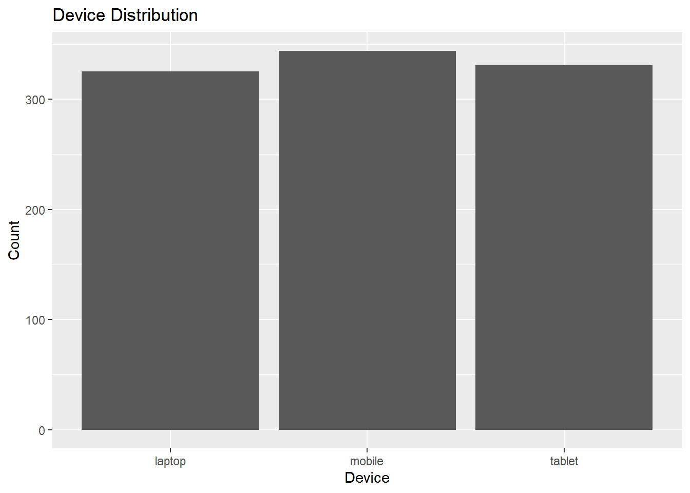
ecom2 %>%
  dbplot::dbplot_bar(device) +
  ggplot2::xlab("Device") +
  ggplot2::ylab("Count") +
  ggplot2::ggtitle("Device Distribution")
Line Chart
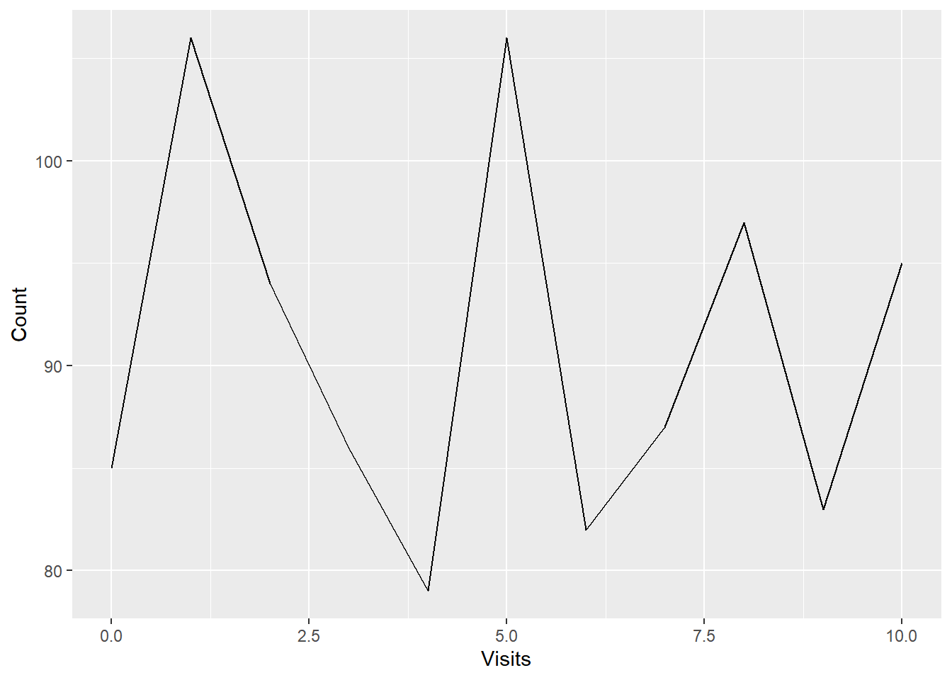
ecom2 %>%
  dbplot::dbplot_line(n_visit) +
  ggplot2::xlab("Visits") +
  ggplot2::ylab("Count")
Your Turn
-
create bar plot of
referrer column from the trade table
-
create line chart of
n_visit column from the trade table
Data Modeling
In this section, we will explore fitting models and running predictions inside the database using the following packages:
Let us start with fitting models inside database. The modeldb package fits models inside database by using dplyr and dbplyr for SQL translation of the algorithms and currently supports linear regression and k-means clustering.
Simple Regression
Let us begin with a simple linear regression model. From the ecom table in the database, we want to regress duration on n_visit. As shown below, we first select the required fields using select() and pass the resulting data to linear_regression_db() from modeldb. We need to specify the dependent variable which in our case is duration.
ecom2 %>%
  dplyr::select(duration, n_visit) %>%
  modeldb::linear_regression_db(duration)
## # A tibble: 1 x 2
##   `(Intercept)` n_visit
##           <dbl>   <dbl>
## 1          364.   -1.72
Let us move on to a multiple regression example. In the below example, we want to regress duration on n_visit (number of visit) and n_pages (number of pages browsed).
Multiple Regression
ecom2 %>%
  dplyr::select(duration, n_visit, n_pages) %>%
  modeldb::linear_regression_db(duration)
## # A tibble: 1 x 3
##   `(Intercept)` n_visit n_pages
##           <dbl>   <dbl>   <dbl>
## 1          415.   -2.02   -8.37
Categorical Variables
So how do we handle categorical variables? To handle categorical variables, use add_dummy_variables(). We need to specify the categorical variable and its values. It will create the dummy variables.
ecom2 %>%
  dplyr::select(duration, device) %>%
  modeldb::add_dummy_variables(device, values = c("laptop", "mobile", "tablet")) %>%
  modeldb::linear_regression_db(duration)
## # A tibble: 1 x 3
##   `(Intercept)` device_mobile device_tablet
##           <dbl>         <dbl>         <dbl>
## 1          376.         -39.2         -22.1
Full Example
Below is a full example, where we have both continuous and categorical predictors. Whenever you have 3 or more predictors, use the sample_size or auto_count arguments. To know why, click here
# use sample size
ecom2 %>%
  dplyr::select(duration, n_visit, n_pages, device) %>%
  modeldb::add_dummy_variables(device, values = c("laptop", "mobile", "tablet")) %>%
  modeldb::linear_regression_db(duration, sample_size = 1000)
## # A tibble: 1 x 5
##   `(Intercept)` n_visit n_pages device_mobile device_tablet
##           <dbl>   <dbl>   <dbl>         <dbl>         <dbl>
## 1          427.   -1.52   -8.27         -31.1         -14.4
# use auto_count
ecom2 %>%
  dplyr::select(duration, n_visit, n_pages, device) %>%
  modeldb::add_dummy_variables(device, values = c("laptop", "mobile", "tablet")) %>%
  modeldb::linear_regression_db(duration, auto_count = TRUE)
## # A tibble: 1 x 5
##   `(Intercept)` n_visit n_pages device_mobile device_tablet
##           <dbl>   <dbl>   <dbl>         <dbl>         <dbl>
## 1          427.   -1.52   -8.27         -31.1         -14.4
Your Turn
-
regress
duration on n_pages
-
regress
duration on referrer
-
and finally regress
duration on n_pages, n_visit and referrer
Predict Inside Database
tidypredict can return SQL statement that can be run inside the database. Let us first create a linear model in R using lm()
model <- lm(duration ~ device + referrer + n_visit + n_pages, data = ecom2)
model
##
## Call:
## lm(formula = duration ~ device + referrer + n_visit + n_pages,
##     data = ecom2)
##
## Coefficients:
##    (Intercept)    devicemobile    devicetablet  referrerdirect  referrergoogle
##        441.450         -30.952         -14.497          -8.980         -10.038
## referrersocial   referreryahoo         n_visit         n_pages
##        -19.841         -32.097          -1.433          -8.298
Fit
To add the fitted values in a new column, use tidypredict_to_column(). In the below example, we use model to compute the fitted values and add it as a new column.
ecom2 %>%
  tidypredict::tidypredict_to_column(model) %>%
  dplyr::select(duration, fit)
## # Source:   lazy query [?? x 2]
## # Database: sqlite 3.30.1 [J:\R\Others\blogs\content\post\mydatabase.db]
##    duration   fit
##       <dbl> <dbl>
##  1      693  409.
##  2      459  374.
##  3      996  424.
##  4      468  273.
##  5      955  357.
##  6      135  361.
##  7       75  356.
##  8      908  379.
##  9      209  249.
## 10      208  384.
## # ... with more rows
tidypredict_fit() returns a Tidy Eval formula that can be used inside a dplyr command.
tidypredict::tidypredict_fit(model)
## 441.450192491919 + (ifelse(device == "mobile", 1, 0) * -30.9522074131866) +
##     (ifelse(device == "tablet", 1, 0) * -14.4972018107797) +
##     (ifelse(referrer == "direct", 1, 0) * -8.98035001912995) +
##     (ifelse(referrer == "google", 1, 0) * -10.038005625893) +
##     (ifelse(referrer == "social", 1, 0) * -19.8411767075006) +
##     (ifelse(referrer == "yahoo", 1, 0) * -32.0969778768984) +
##     (n_visit * -1.4325653130794) + (n_pages * -8.29825840984566)
Let us use the above R code to calculate fitted values using mutate() from dplyr.
ecom2 %>%
  dplyr::mutate(
    fit = 441.450192491919 + (ifelse(device == "mobile", 1, 0) *
      -30.9522074131866) + (ifelse(device == "tablet", 1,
      0) * -14.4972018107797) + (ifelse(referrer == "direct",
      1, 0) * -8.98035001912995) + (ifelse(referrer == "google",
      1, 0) * -10.038005625893) + (ifelse(referrer == "social",
      1, 0) * -19.8411767075006) + (ifelse(referrer == "yahoo",
      1, 0) * -32.0969778768984) + (n_visit * -1.4325653130794) +
      (n_pages * -8.29825840984566)
    ) %>%
  dplyr::select(duration, fit)
## # Source:   lazy query [?? x 2]
## # Database: sqlite 3.30.1 [J:\R\Others\blogs\content\post\mydatabase.db]
##    duration   fit
##       <dbl> <dbl>
##  1      693  409.
##  2      459  374.
##  3      996  424.
##  4      468  273.
##  5      955  357.
##  6      135  361.
##  7       75  356.
##  8      908  379.
##  9      209  249.
## 10      208  384.
## # ... with more rows
The SQL translation of the above step can be viewed using tidypredict_sql().
tidypredict::tidypredict_sql(model, con)
## <SQL> 441.450192491919 + (CASE WHEN (`device` = 'mobile') THEN (1.0) WHEN NOT(`device` = 'mobile') THEN (0.0) END * -30.9522074131866) + (CASE WHEN (`device` = 'tablet') THEN (1.0) WHEN NOT(`device` = 'tablet') THEN (0.0) END * -14.4972018107797) + (CASE WHEN (`referrer` = 'direct') THEN (1.0) WHEN NOT(`referrer` = 'direct') THEN (0.0) END * -8.98035001912995) + (CASE WHEN (`referrer` = 'google') THEN (1.0) WHEN NOT(`referrer` = 'google') THEN (0.0) END * -10.038005625893) + (CASE WHEN (`referrer` = 'social') THEN (1.0) WHEN NOT(`referrer` = 'social') THEN (0.0) END * -19.8411767075006) + (CASE WHEN (`referrer` = 'yahoo') THEN (1.0) WHEN NOT(`referrer` = 'yahoo') THEN (0.0) END * -32.0969778768984) + (`n_visit` * -1.4325653130794) + (`n_pages` * -8.29825840984566)
Close Connection
It is a good practice to close connection to a database when you no longer need to read/write data from/to it. Use dbDisconnect() to close the database connection.
DBI::dbDisconnect(con)

RStudio Connections Pane
In this section, we will learn to connect and explore databases using RStudio connections pane. We will connect to a MySQL database hosted on AWS. For security reasons, the database will be deleted after this post has been published and you will not be able to reproduce the results from this section onwards. Now, in the below images we show how to add and explore a new connection. The Connections Pane is available only in RStudio 1.1 and later.
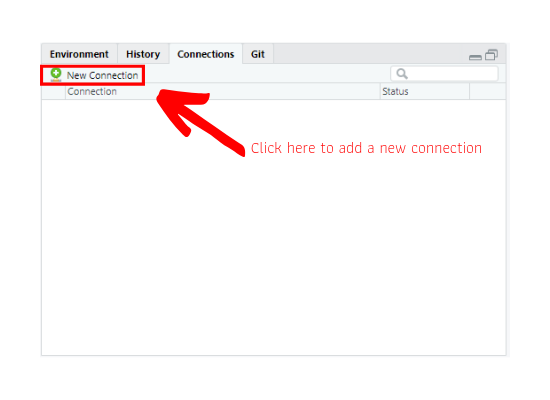
Step 1: Click on New Connection
In the Connections Pane, click on the New Connection button.
Step 2: Connect to a Data Source
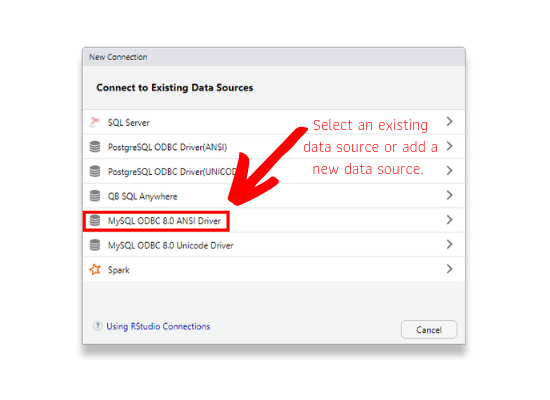
Once you click on New Connection, RStudio will display the exisiting data sources. If you do not see the driver for the database you want to connect to, install the driver and check again. Visit https://db.rstudio.com/best-practices/drivers/ for more information about setting up ODBC drivers.
Step 3: Supply Database Connection Parameters
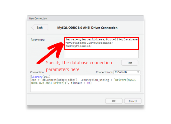
If the database driver is already present, click on it to create a new connection. Specify the database parameters in the text box as shown in the below image. Visit https://www.connectionstrings.com/ to learn how to specify the connection strings for different databases.
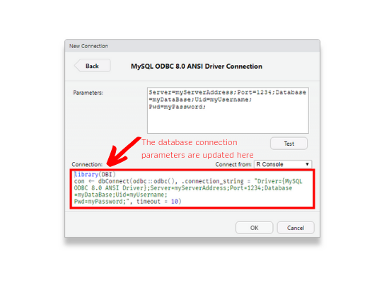
Once you specify the database parameters, the R code will be automatically updated by RStudio as shown below.
Step 4: Test Connection
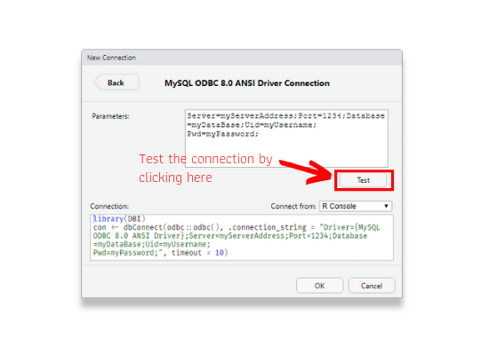
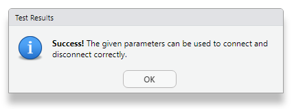
After specifying the database connection parameters, we can test if the connection works by clicking on Test.
If RStudio is able to connect to the database, it will show a success message as shown below.
Step 5: Connect Options
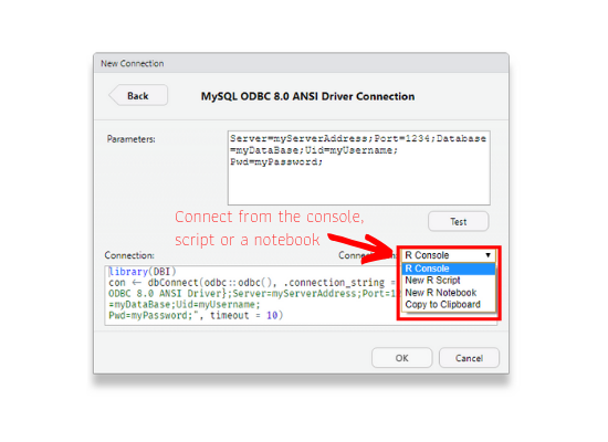
After testing the connection, you can choose to connect from
-
the console
-
R script
-
or a notebook.
You can copy the R code to the clipboard as well. Depending on where you intend to use the connection i.e. interactive session, R script or notebook, choose the appropriate option.
Step 6: Open New Connection
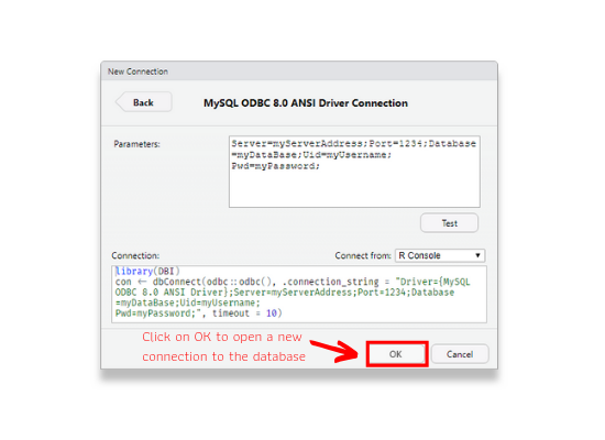
Click on OK button to open a new connection to the database.
Step 7: Explore Database
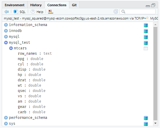
You can explore the database from the Connections tab. View the tables in the database, explore the fields in a table, open a SQL script to run queries or close the connection if you don’t need it any longer.
Handling Credentials
Handling database credentials is one of the most important part of working with databases in R. In this section, we will look at the different options for securely storing and accessing credentials. After connecting to the database, we will list the tables in the database (just to check that the connection is working) and then disconnect.
rstudioapi
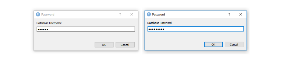
You can prompt the user to enter the database credentials using RStudio IDE. askForPassword() will show a popup box that masks what is typed.
db_con <- DBI::dbConnect(drv      = RMySQL::MySQL(),
                         username = rstudioapi::askForPassword("Database Username"),
                         password = rstudioapi::askForPassword("Database Password"),
                         host     = "mysql-ecom.cowqoftkc0gy.us-east-2.rds.amazonaws.com",
                         port     = 3306,
                         dbname   = "mysql_test")
.Renviron
The second method is store the credentials as environment variables. This can be achieved using Sys.setenv() or using .Renviron file. The credentials can then be retrieved using Sys.getenv() as shown in the below example:
db_con <- DBI::dbConnect(drv      = RMySQL::MySQL(),
                         username = Sys.getenv("db_uid"),
                         password = Sys.getenv("db_pwd"),
                         host     = "mysql-ecom.cowqoftkc0gy.us-east-2.rds.amazonaws.com",
                         port     = 3306,
                         dbname   = "mysql_test")

# list tables in the database
DBI::dbListTables(db_con)
DBI::dbDisconnect(db_con)
In RStudio, create a new file and save it as .Renviron. In this file, define the credentials as shown below:
userid = "username"
pwd    = "password"
Save the file in the home directory of your project and restart R. Why should you restart R? .Renviron is processed only at the beginning of an R session. If you try to access the credentials using Sys.getenv() without restarting R, the credentials will not be retrieved and you will see an error if you try to connect to the database. After restarting R, use Sys.getenv() to retrieve the credentials while opening a new connection to the database. We have added the .Renviron file used to store credentials in the resources section of the learning management system as well as in the GitHub repo.
options
The database credentials can be recorded as a global option in R. There are two ways to do this:
-
use
options()
-
use an R file
Below is the code that records credentials using options():
options(db_userid   = "user_id")
options(db_password = "pass_word")
The above code can be stored in a R file which can then be sourced before opening a new connection to the database. The credentials can be retrieved using getOptions(). We have added the options.R file used to store credentials to the database in the resources section of the learning management system as well as in the GitHub repo.
source("options.R")
db_con <- DBI::dbConnect(drv      = RMySQL::MySQL(),
                         username = getOption("db_userid"),
                         password = getOption("db_password"),
                         host     = "mysql-ecom.cowqoftkc0gy.us-east-2.rds.amazonaws.com",
                         port     = 3306,
                         dbname   = "mysql_test")

# list tables in the database
DBI::dbListTables(db_con)
DBI::dbDisconnect(db_con)
config
The config package allows you to manage environment specific configuration values. Configurations are defined using a YAML text file and are read by default from a file named config.yml in the current working directory. Store the database connection details such as driver, username, password, host, port, database name etc. in a YAML file and read it using get(). We have added the config.yml file used to store the credentials in the resources section of the learning management system as well as in the GitHub repo.
# read configurations
md <- config::get("mysql-dev")

# test
md$port
md$dbname

# connect
db_con <- DBI::dbConnect(drv      = RMySQL::MySQL(),
                         username = md$username,
                         password = md$password,
                         host     = md$host,
                         port     = md$port,
                         dbname   = md$dbname)

# list tables in the database
DBI::dbListTables(db_con)
DBI::dbDisconnect(db_con)
keyring
The keyring package provides platform independent API to access the operating systems credential store. We leave it to the reader to explore the keyring package for storing and accessing credentials safely.
dbx
dbx is another interesting package built on top of DBI for both research and production environments and we hope to explore it in a separate post in the coming days.
Summary
-
DBI to connect and interact with databases
-
dplyr and dbplyr for data transformation
-
dbplot for data visualization
-
modeldb and tidypredict for data modeling
-
config, keyring, .Renviron and
options() to handle credentials
-
always close the database connection