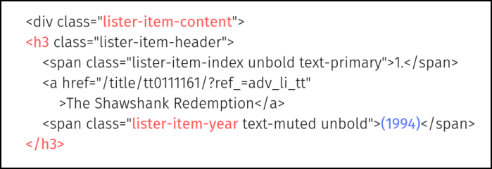
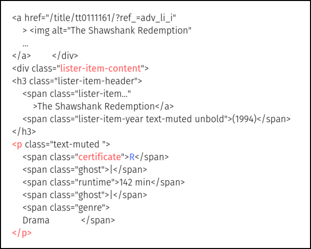
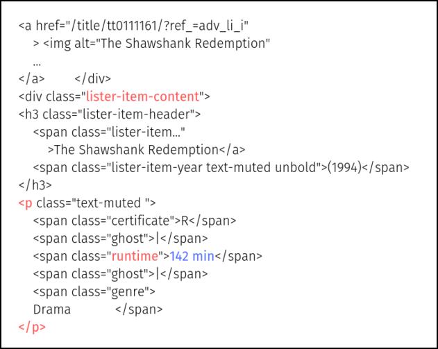
In this case study, we will extract the following details of the top 50 movies from the IMDB website:
Genre
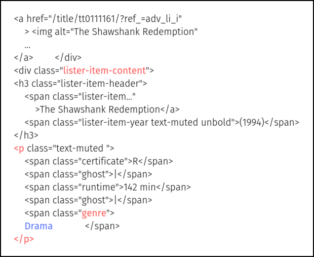
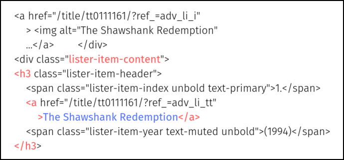
The genre of the movie can be located in the following way:
-
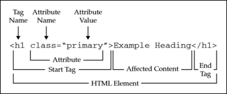
<span> tag identified by the class .genre
-
nested inside a paragraph (
<p>)
-
part of section identified by the class
.lister-item-content
imdb %>%
  html_nodes(".lister-item-content p .genre") %>%
  html_text()
##  [1] "\nDrama            "
##  [2] "\nCrime, Drama            "
##  [3] "\nAction, Crime, Drama            "
##  [4] "\nCrime, Drama            "
##  [5] "\nAdventure, Drama, Fantasy            "
##  [6] "\nCrime, Drama            "
##  [7] "\nBiography, Drama, History            "
##  [8] "\nCrime, Drama            "
##  [9] "\nAction, Adventure, Sci-Fi            "
## [10] "\nDrama            "
## [11] "\nAction, Adventure, Drama            "
## [12] "\nDrama, Romance            "
## [13] "\nWestern            "
## [14] "\nAdventure, Drama, Fantasy            "
## [15] "\nAction, Sci-Fi            "
## [16] "\nBiography, Crime, Drama            "
## [17] "\nAction, Adventure, Fantasy            "
## [18] "\nDrama            "
## [19] "\nAction, Drama, History            "
## [20] "\nComedy, Drama, Thriller            "
## [21] "\nAdventure, Drama, Sci-Fi            "
## [22] "\nCrime, Drama            "
## [23] "\nAnimation, Adventure, Family            "
## [24] "\nDrama, War            "
## [25] "\nCrime, Drama, Fantasy            "
## [26] "\nComedy, Drama, Romance            "
## [27] "\nCrime, Drama, Mystery            "
## [28] "\nCrime, Drama, Thriller            "
## [29] "\nAction, Adventure, Fantasy            "
## [30] "\nDrama, Musical            "
## [31] "\nAction, Adventure, Drama            "
## [32] "\nDrama, Family, Fantasy            "
## [33] "\nCrime, Drama, Thriller            "
## [34] "\nAction, Adventure, Sci-Fi            "
## [35] "\nDrama, Music            "
## [36] "\nBiography, Comedy, Drama            "
## [37] "\nDrama, Mystery, Sci-Fi            "
## [38] "\nCrime, Drama, Thriller            "
## [39] "\nBiography, Drama, Music            "
## [40] "\nAction, Adventure, Drama            "
## [41] "\nDrama            "
## [42] "\nCrime, Mystery, Thriller            "
## [43] "\nAction, Crime, Drama            "
## [44] "\nAnimation, Adventure, Drama            "
## [45] "\nAction, Sci-Fi            "
## [46] "\nDrama            "
## [47] "\nAnimation, Drama, War            "
## [48] "\nAdventure, Comedy, Sci-Fi            "
## [49] "\nWestern            "
## [50] "\nCrime, Drama, Mystery            "
The output includes str_trim().
imdb %>%
  html_nodes(".lister-item-content p .genre") %>%
  html_text() %>%
  str_trim() -> movie_genre

movie_genre
##  [1] "Drama"                        "Crime, Drama"
##  [3] "Action, Crime, Drama"         "Crime, Drama"
##  [5] "Adventure, Drama, Fantasy"    "Crime, Drama"
##  [7] "Biography, Drama, History"    "Crime, Drama"
##  [9] "Action, Adventure, Sci-Fi"    "Drama"
## [11] "Action, Adventure, Drama"     "Drama, Romance"
## [13] "Western"                      "Adventure, Drama, Fantasy"
## [15] "Action, Sci-Fi"               "Biography, Crime, Drama"
## [17] "Action, Adventure, Fantasy"   "Drama"
## [19] "Action, Drama, History"       "Comedy, Drama, Thriller"
## [21] "Adventure, Drama, Sci-Fi"     "Crime, Drama"
## [23] "Animation, Adventure, Family" "Drama, War"
## [25] "Crime, Drama, Fantasy"        "Comedy, Drama, Romance"
## [27] "Crime, Drama, Mystery"        "Crime, Drama, Thriller"
## [29] "Action, Adventure, Fantasy"   "Drama, Musical"
## [31] "Action, Adventure, Drama"     "Drama, Family, Fantasy"
## [33] "Crime, Drama, Thriller"       "Action, Adventure, Sci-Fi"
## [35] "Drama, Music"                 "Biography, Comedy, Drama"
## [37] "Drama, Mystery, Sci-Fi"       "Crime, Drama, Thriller"
## [39] "Biography, Drama, Music"      "Action, Adventure, Drama"
## [41] "Drama"                        "Crime, Mystery, Thriller"
## [43] "Action, Crime, Drama"         "Animation, Adventure, Drama"
## [45] "Action, Sci-Fi"               "Drama"
## [47] "Animation, Drama, War"        "Adventure, Comedy, Sci-Fi"
## [49] "Western"                      "Crime, Drama, Mystery"
Rating
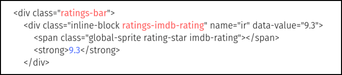
The rating of the movie can be located in the following way:
-
part of the section identified by the class
.ratings-imdb-rating
-
nested within the section identified by the class
.ratings-bar
-
the rating is present within the
<strong> tag as well as in the data-value attribute
-
instead of using
html_text(), we will use html_attr() to extract the value of the attribute data-value
Try using html_text() and see what happens! You may include the <strong> tag or the classes associated with <span> tag as well.
imdb %>%
  html_nodes(".ratings-bar .ratings-imdb-rating") %>%
  html_attr("data-value")
##  [1] "9.3" "9.2" "9"   "9"   "8.9" "8.9" "8.9" "8.9" "8.8" "8.8" "8.8" "8.8"
## [13] "8.8" "8.7" "8.7" "8.7" "8.7" "8.7" "8.7" "8.6" "8.6" "8.6" "8.6" "8.6"
## [25] "8.6" "8.6" "8.6" "8.6" "8.6" "8.6" "8.6" "8.6" "8.5" "8.5" "8.5" "8.5"
## [37] "8.5" "8.5" "8.5" "8.5" "8.5" "8.5" "8.5" "8.5" "8.5" "8.5" "8.5" "8.5"
## [49] "8.5" "8.5"
Since rating is returned as a character vector, we will use as.numeric() to convert it into a number.
imdb %>%
  html_nodes(".ratings-bar .ratings-imdb-rating") %>%
  html_attr("data-value") %>%
  as.numeric() -> movie_rating

movie_rating
##  [1] 9.3 9.2 9.0 9.0 8.9 8.9 8.9 8.9 8.8 8.8 8.8 8.8 8.8 8.7 8.7 8.7 8.7 8.7 8.7
## [20] 8.6 8.6 8.6 8.6 8.6 8.6 8.6 8.6 8.6 8.6 8.6 8.6 8.6 8.5 8.5 8.5 8.5 8.5 8.5
## [39] 8.5 8.5 8.5 8.5 8.5 8.5 8.5 8.5 8.5 8.5 8.5 8.5

XPATH
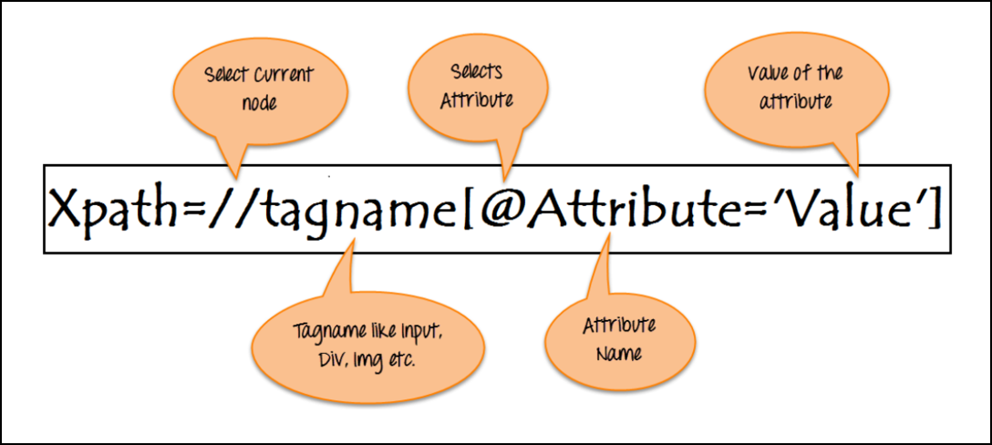
To extract votes from the web page, we will use a different technique. In this case, we will use xpath and attributes to locate the total number of votes received by the top 50 movies.
xpath is specified using the following:
-
tab
-
attribute name
-
attribute value
Votes
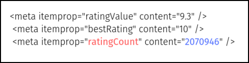 In case of votes, they are the following:
-
meta
-
itemprop
-
ratingCount
Next, we are not looking to extract text value as we did in the previous examples using html_text(). Here, we need to extract the value assigned to the content attribute within the <meta> tag using html_attr().
imdb %>%
  html_nodes(xpath = '//meta[@itemprop="ratingCount"]') %>%
  html_attr('content')
##  [1] "2249246" "1552001" "2217242" "1084778" "1588695" "1761054" "1168838"
##  [8] "658477"  "1972065" "1788415" "1602475" "1734160" "664323"  "1435345"
## [15] "1613462" "978543"  "1121218" "881910"  "34773"   "424531"  "1422868"
## [22] "679953"  "614374"  "1189533" "1096715" "598021"  "1384558" "1217882"
## [29] "1193648" "26469"   "303892"  "383949"  "806007"  "779460"  "679324"
## [36] "728348"  "1139520" "1146357" "698328"  "1293047" "1004432" "958513"
## [43] "995573"  "906648"  "965426"  "218874"  "220345"  "1008251" "290832"
## [50] "29464"
Finally, we convert the votes to a number using as.numeric().
imdb %>%
  html_nodes(xpath = '//meta[@itemprop="ratingCount"]') %>%
  html_attr('content') %>%
  as.numeric() -> movie_votes

movie_votes
##  [1] 2249246 1552001 2217242 1084778 1588695 1761054 1168838  658477 1972065
## [10] 1788415 1602475 1734160  664323 1435345 1613462  978543 1121218  881910
## [19]   34773  424531 1422868  679953  614374 1189533 1096715  598021 1384558
## [28] 1217882 1193648   26469  303892  383949  806007  779460  679324  728348
## [37] 1139520 1146357  698328 1293047 1004432  958513  995573  906648  965426
## [46]  218874  220345 1008251  290832   29464
Revenue
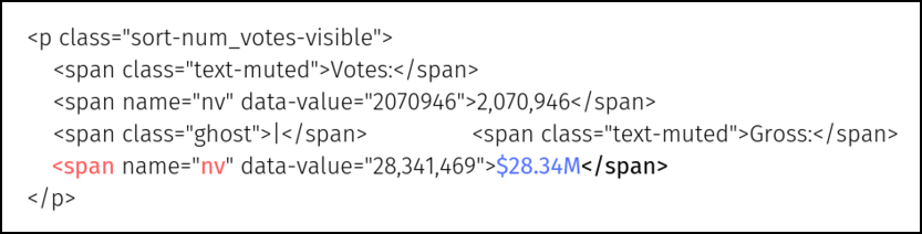
We wanted to extract both revenue and votes without using xpath but the way in which they are structured in the HTML code forced us to use xpath to extract votes. If you look at the HTML code, both votes and revenue are located inside the same tag with the same attribute name and value i.e. there is no distinct way to identify either of them.
In case of revenue, the xpath details are as follows:
Next, we will use html_text() to extract the revenue.
imdb %>%
  html_nodes(xpath = '//span[@name="nv"]') %>%
  html_text()
##  [1] "2,249,246" "$28.34M"   "1,552,001" "$134.97M"  "2,217,242" "$534.86M"
##  [7] "1,084,778" "$57.30M"   "1,588,695" "$377.85M"  "1,761,054" "$107.93M"
## [13] "1,168,838" "$96.90M"   "658,477"   "$4.36M"    "1,972,065" "$292.58M"
## [19] "1,788,415" "$37.03M"   "1,602,475" "$315.54M"  "1,734,160" "$330.25M"
## [25] "664,323"   "$6.10M"    "1,435,345" "$342.55M"  "1,613,462" "$171.48M"
## [31] "978,543"   "$46.84M"   "1,121,218" "$290.48M"  "881,910"   "$112.00M"
## [37] "34,773"    "424,531"   "$53.37M"   "1,422,868" "$188.02M"  "679,953"
## [43] "$7.56M"    "614,374"   "$10.06M"   "1,189,533" "$216.54M"  "1,096,715"
## [49] "$136.80M"  "598,021"   "$57.60M"   "1,384,558" "$100.13M"  "1,217,882"
## [55] "$130.74M"  "1,193,648" "$322.74M"  "26,469"    "303,892"   "$0.27M"
## [61] "383,949"   "806,007"   "$335.45M"  "779,460"   "$678.82M"  "679,324"
## [67] "$13.09M"   "728,348"   "$13.18M"   "1,139,520" "$53.09M"   "1,146,357"
## [73] "$132.38M"  "698,328"   "$32.57M"   "1,293,047" "$187.71M"  "1,004,432"
## [79] "$6.72M"    "958,513"   "$23.34M"   "995,573"   "$19.50M"   "906,648"
## [85] "$422.78M"  "965,426"   "$204.84M"  "218,874"   "$11.99M"   "220,345"
## [91] "1,008,251" "$210.61M"  "290,832"   "$5.32M"    "29,464"
To extract the revenue as a number, we need to do some string hacking as follows:
-
extract values that begin with
\(</code></li>
<li>omit missing values</li>
<li>convert values to character using <code>as.character()</code></li>
<li>append NA where revenue is missing (rank 31 and 47)</li>
<li>remove <code>\)
and M
-
convert to number using
as.numeric()
imdb %>%
  html_nodes(xpath = '//span[@name="nv"]') %>%
  html_text() %>%
  str_extract(pattern = "^\\$.*") %>%
  na.omit() %>%
  as.character() %>%
  append(values = NA, after = 18) %>%
  append(values = NA, after = 29) %>%
  append(values = NA, after = 31) %>%
  append(values = NA, after = 46) %>%
  append(values = NA, after = 49) %>%
  str_sub(start = 2, end = nchar(.) - 1) %>%
  as.numeric() -> movie_revenue

movie_revenue
##  [1]  28.34 134.97 534.86  57.30 377.85 107.93  96.90   4.36 292.58  37.03
## [11] 315.54 330.25   6.10 342.55 171.48  46.84 290.48 112.00     NA  53.37
## [21] 188.02   7.56  10.06 216.54 136.80  57.60 100.13 130.74 322.74     NA
## [31]   0.27     NA 335.45 678.82  13.09  13.18  53.09 132.38  32.57 187.71
## [41]   6.72  23.34  19.50 422.78 204.84  11.99     NA 210.61   5.32     NA
Putting it all together…
top_50 <- tibble(title = movie_title, release = movie_year,
    `runtime (mins)` = movie_runtime, genre = movie_genre, rating = movie_rating,
    votes = movie_votes, `revenue ($ millions)` = movie_revenue)

top_50
## # A tibble: 50 x 7
##    title       release `runtime (mins)` genre    rating   votes `revenue ($ mil~
##    <chr>         <dbl>            <dbl> <chr>     <dbl>   <dbl>            <dbl>
##  1 The Shawsh~    1994              142 Drama       9.3 2249246            28.3
##  2 The Godfat~    1972              175 Crime, ~    9.2 1552001           135.
##  3 The Dark K~    2008              152 Action,~    9   2217242           535.
##  4 The Godfat~    1974              202 Crime, ~    9   1084778            57.3
##  5 The Lord o~    2003              201 Adventu~    8.9 1588695           378.
##  6 Pulp Ficti~    1994              154 Crime, ~    8.9 1761054           108.
##  7 Schindler'~    1993              195 Biograp~    8.9 1168838            96.9
##  8 12 Angry M~    1957               96 Crime, ~    8.9  658477             4.36
##  9 Inception      2010              148 Action,~    8.8 1972065           293.
## 10 Fight Club     1999              139 Drama       8.8 1788415            37.0
## # ... with 40 more rows

Top Websites
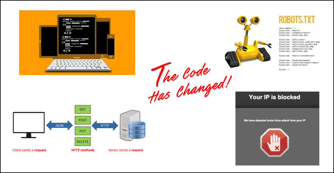
Unfortunately, we had to drop this case study as the HTML code changed while we were working on this blog post. Remember, the third point we mentioned in the things to keep in mind, where we had warned that the design or underlying HTML code of the website may change. It just happened as we were finalizing this post.
RBI Governors
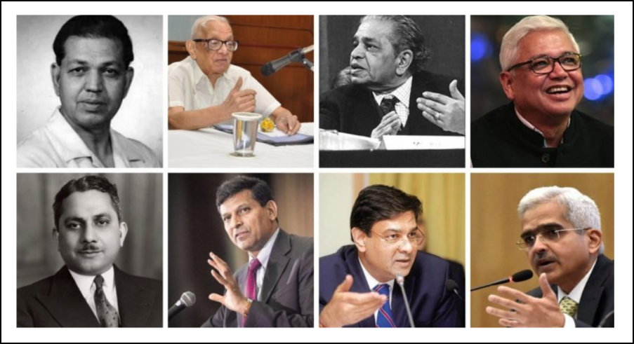
In this case study, we are going to extract the list of RBI (Reserve Bank of India) Governors. The author of this blog post comes from an Economics background and as such was intereseted in knowing the professional background of the Governors prior to their taking charge at India’s central bank. We will extact the following details:
-
name
-
start of term
-
end of term
-
term (in days)
-
background
robotstxt
Let us check if we can scrape the data from Wikipedia website using paths_allowed() from robotstxt package.
paths_allowed(
  paths = c("https://en.wikipedia.org/wiki/List_of_Governors_of_Reserve_Bank_of_India")
)
##
 en.wikipedia.org
## [1] TRUE
Since it has returned TRUE, we will go ahead and download the web page using read_html() from xml2 package.
rbi_guv <- read_html("https://en.wikipedia.org/wiki/List_of_Governors_of_Reserve_Bank_of_India")
rbi_guv
## {html_document}
## <html class="client-nojs" lang="en" dir="ltr">
## [1] <head>\n<meta http-equiv="Content-Type" content="text/html; charset=UTF-8 ...
## [2] <body class="mediawiki ltr sitedir-ltr mw-hide-empty-elt ns-0 ns-subject  ...
List of Governors
The data in the Wikipedia page is luckily structured as a table and we can extract it using html_table().
rbi_guv %>%
  html_nodes("table") %>%
  html_table()
## [[1]]
## Governor of the Reserve Bank of India
## 1 IncumbentShaktikanta Das, IASsince 12 December 2018; 17 months ago (2018-12-12)
## 2 Appointer
## 3 Term length
## 4 Constituting instrument
## 5 Inaugural holder
## 6 Formation
## 7 Deputy
## 8 Salary
## 9 Website
## Governor of the Reserve Bank of India
## 1 IncumbentShaktikanta Das, IASsince 12 December 2018; 17 months ago (2018-12-12)
## 2 President of India
## 3 Three years
## 4 Reserve Bank of India Act, 1934
## 5 Osborne Smith (1935–1937)
## 6 1 April 1935; 85 years ago (1935-04-01)
## 7 Deputy Governors of the Reserve Bank of India
## 8 <U+20B9> 2,50,000
## 9 rbi.org.in
##
## [[2]]
## No. Officeholder Portrait Term start Term end
## 1 1 Osborne Smith NA 1 April 1935 30 June 1937
## 2 2 James Braid Taylor NA 1 July 1937 17 February 1943
## 3 3 C. D. Deshmukh NA 11 August 1943 30 June 1949
## 4 4 Benegal Rama Rau NA 1 July 1949 14 January 1957
## 5 5 K. G. Ambegaonkar NA 14 January 1957 28 February 1957
## 6 6 H. V. R. Iyengar NA 1 March 1957 28 February 1962
## 7 7 P. C. Bhattacharya NA 1 March 1962 30 June 1967
## 8 8 Lakshmi Kant Jha NA 1 July 1967 3 May 1970
## 9 9 B. N. Adarkar NA 4 May 1970 15 June 1970
## 10 10 Sarukkai Jagannathan NA 16 June 1970 19 May 1975
## 11 11 N. C. Sen Gupta NA 19 May 1975 19 August 1975
## 12 12 K. R. Puri NA 20 August 1975 2 May 1977
## 13 13 M. Narasimham NA 3 May 1977 30 November 1977
## 14 14 I. G. Patel NA 1 December 1977 15 September 1982
## 15 15 Manmohan Singh NA 16 September 1982 14 January 1985
## 16 16 Amitav Ghosh NA 15 January 1985 4 February 1985
## 17 17 R. N. Malhotra NA 4 February 1985 22 December 1990
## 18 18 S. Venkitaramanan NA 22 December 1990 21 December 1992
## 19 19 C. Rangarajan NA 22 December 1992 21 November 1997
## 20 20 Bimal Jalan NA 22 November 1997 6 September 2003
## 21 21 Y. Venugopal Reddy NA 6 September 2003 5 September 2008
## 22 22 D. Subbarao NA 5 September 2008 4 September 2013
## 23 23 Raghuram Rajan NA 4 September 2013 4 September 2016
## 24 24 Urjit Patel NA 4 September 2016 11 December 2018
## 25 25 Shaktikanta Das NA 12 December 2018 Incumbent
## Term in office Background
## 1 821 days Banker
## 2 2057 days Indian Civil Service (ICS) officer
## 3 2150 days ICS officer
## 4 2754 days ICS officer
## 5 45 days ICS officer
## 6 1825 days ICS officer
## 7 1947 days Indian Audit and Accounts Service officer
## 8 1037 days ICS officer
## 9 42 days Economist
## 10 1798 days ICS officer
## 11 92 days ICS officer
## 12 621 days
## 13 211 days Career Reserve Bank of India officer
## 14 1749 days Economist
## 15 851 days Economist
## 16 20 days Banker
## 17 2147 days Indian Administrative Service (IAS) officer
## 18 730 days IAS officer
## 19 1795 days Economist
## 20 2114 days Economist
## 21 1826 days IAS officer
## 22 1825 days IAS officer
## 23 1096 days Economist
## 24 828 days Economist
## 25 540 days IAS officer
## Prior office(s)
## 1 Managing Governor of the Imperial Bank of India
## 2 Deputy Governor of the Reserve Bank of India\n\nController of Currency
## 3 Deputy Governor of the Reserve Bank of India\nCustodian of Enemy Property
## 4 Ambassador of India to the United States\n\nAmbassador of India to Japan\n\nChairman of Bombay Port Trust
## 5 Finance Secretary
## 6 Chairman of the State Bank of India
## 7 Chairman of the State Bank of India\nSecretary in the Ministry of Finance
## 8 Secretary to the Prime Minister of India
## 9 Executive Director at the International Monetary Fund
## 10 Executive Director at the World Bank
## 11 Banking Secretary
## 12 Chairman and Managing Director of the Life Insurance Corporation
## 13 Deputy Governor of the Reserve Bank of India
## 14 Director of the London School of Economics\n\nDeputy Administrator of the United Nations Development Programme\nChief Economic Adviser to the Government of India
## 15 Secretary in the Ministry of Finance\n\nChief Economic Adviser to the Government of India
## 16 Deputy Governor of the Reserve Bank of India\n\nChairman of the Allahabad Bank
## 17 Finance Secretary\n\nExecutive Director at the International Monetary Fund
## 18 Finance Secretary
## 19 Deputy Governor of the Reserve Bank of India
## 20 Finance Secretary\n\nBanking Secretary\n\nChief Economic Adviser to the Government of India
## 21 Executive Director at the International Monetary Fund\n\nDeputy Governor of the Reserve Bank of India
## 22 Finance Secretary\n\nMember-Secretary of the Prime Minister's Economic Advisory Council
## 23 Chief Economic Adviser to the Government of India\nChief Economist of International Monetary Fund
## 24 Deputy Governor of the Reserve Bank
## 25 Member of the Fifteenth Finance Commission\nSherpa of India to the G20\nEconomic Affairs Secretary\nRevenue Secretary
## Reference(s)
## 1 [2]
## 2 [3]
## 3
## 4
## 5
## 6
## 7
## 8
## 9
## 10
## 11
## 12
## 13
## 14
## 15
## 16
## 17
## 18
## 19
## 20
## 21
## 22
## 23
## 24
## 25 [4][5][6]
##
## [[3]]
## vte Governors of the Reserve Bank of India
## 1 NA
## vte Governors of the Reserve Bank of India
## 1 Osborne Smith (1935–37)\nJames Braid Taylor (1937–43)\nC. D. Deshmukh (1943–49)\nBenegal Rama Rau (1949–57)\nK. G. Ambegaonkar (1957)\nH. V. R. Iyengar (1957–62)\nP. C. Bhattacharya (1962–67)\nLakshmi Kant Jha (1967–70)\nB. N. Adarkar (1970)\nS. Jagannathan (1970–75)\nN. C. Sen Gupta (1975)\nK. R. Puri (1975–77)\nM. Narasimham (1977)\nI. G. Patel (1977–82)\nManmohan Singh (1982–85)\nAmitav Ghosh (1985)\nR. N. Malhotra (1985–90)\nS. Venkitaramanan (1990–92)\nC. Rangarajan (1992–97)\nBimal Jalan (1997–2003)\nY. Venugopal Reddy (2003–08)\nDuvvuri Subbarao (2008–13)\nRaghuram Rajan (2013–16)\nUrjit Patel (2016–2018)\nShaktikanta Das (2018–Incumbent)
## vte Governors of the Reserve Bank of India
## 1 Osborne Smith (1935–37)\nJames Braid Taylor (1937–43)\nC. D. Deshmukh (1943–49)\nBenegal Rama Rau (1949–57)\nK. G. Ambegaonkar (1957)\nH. V. R. Iyengar (1957–62)\nP. C. Bhattacharya (1962–67)\nLakshmi Kant Jha (1967–70)\nB. N. Adarkar (1970)\nS. Jagannathan (1970–75)\nN. C. Sen Gupta (1975)\nK. R. Puri (1975–77)\nM. Narasimham (1977)\nI. G. Patel (1977–82)\nManmohan Singh (1982–85)\nAmitav Ghosh (1985)\nR. N. Malhotra (1985–90)\nS. Venkitaramanan (1990–92)\nC. Rangarajan (1992–97)\nBimal Jalan (1997–2003)\nY. Venugopal Reddy (2003–08)\nDuvvuri Subbarao (2008–13)\nRaghuram Rajan (2013–16)\nUrjit Patel (2016–2018)\nShaktikanta Das (2018–Incumbent)
## vte Governors of the Reserve Bank of India
## 1 NA
There are 2 tables in the web page and we are interested in the second table. Using extract2() from the magrittr package, we will extract the table containing the details of the Governors.
rbi_guv %>%
  html_nodes("table") %>%
  html_table() %>%
  extract2(2) -> profile
Sort
Let us arrange the data by number of days served. The Term in office column contains this information but it also includes the text days. Let us split this column into two columns, term and days, using separate() from tidyr and then select the columns Officeholder and term and arrange it in descending order using desc().
profile %>%
  separate(`Term in office`, into = c("term", "days")) %>%
  select(Officeholder, term) %>%
  arrange(desc(as.numeric(term)))
##            Officeholder term
## 1      Benegal Rama Rau 2754
## 2        C. D. Deshmukh 2150
## 3        R. N. Malhotra 2147
## 4           Bimal Jalan 2114
## 5    James Braid Taylor 2057
## 6    P. C. Bhattacharya 1947
## 7    Y. Venugopal Reddy 1826
## 8      H. V. R. Iyengar 1825
## 9           D. Subbarao 1825
## 10 Sarukkai Jagannathan 1798
## 11        C. Rangarajan 1795
## 12          I. G. Patel 1749
## 13       Raghuram Rajan 1096
## 14     Lakshmi Kant Jha 1037
## 15       Manmohan Singh  851
## 16          Urjit Patel  828
## 17        Osborne Smith  821
## 18    S. Venkitaramanan  730
## 19           K. R. Puri  621
## 20      Shaktikanta Das  540
## 21        M. Narasimham  211
## 22      N. C. Sen Gupta   92
## 23    K. G. Ambegaonkar   45
## 24        B. N. Adarkar   42
## 25         Amitav Ghosh   20
Backgrounds
What we are interested is in the background of the Governors? Use count() from dplyr to look at the backgound of the Governors and the respective counts.
profile %>%
  count(Background)
##                                    Background n
## 1                                             1
## 2                                      Banker 2
## 3        Career Reserve Bank of India officer 1
## 4                                   Economist 7
## 5                                 IAS officer 4
## 6                                 ICS officer 7
## 7 Indian Administrative Service (IAS) officer 1
## 8   Indian Audit and Accounts Service officer 1
## 9          Indian Civil Service (ICS) officer 1
Let us club some of the categories into Bureaucrats as they belong to the Indian Administrative/Civil Services. The missing data will be renamed as No Info. The category Career Reserve Bank of India officer is renamed as RBI Officer to make it more concise.
profile %>%
  pull(Background) %>%
  fct_collapse(
    Bureaucrats = c("IAS officer", "ICS officer",
    "Indian Administrative Service (IAS) officer",
    "Indian Audit and Accounts Service officer",
    "Indian Civil Service (ICS) officer"),
    `No Info` = c(""),
    `RBI Officer` = c("Career Reserve Bank of India officer")
  ) %>%
  fct_count() %>%
  rename(background = f, count = n) -> backgrounds

backgrounds
## # A tibble: 5 x 2
##   background  count
##   <fct>       <int>
## 1 No Info         1
## 2 Banker          2
## 3 RBI Officer     1
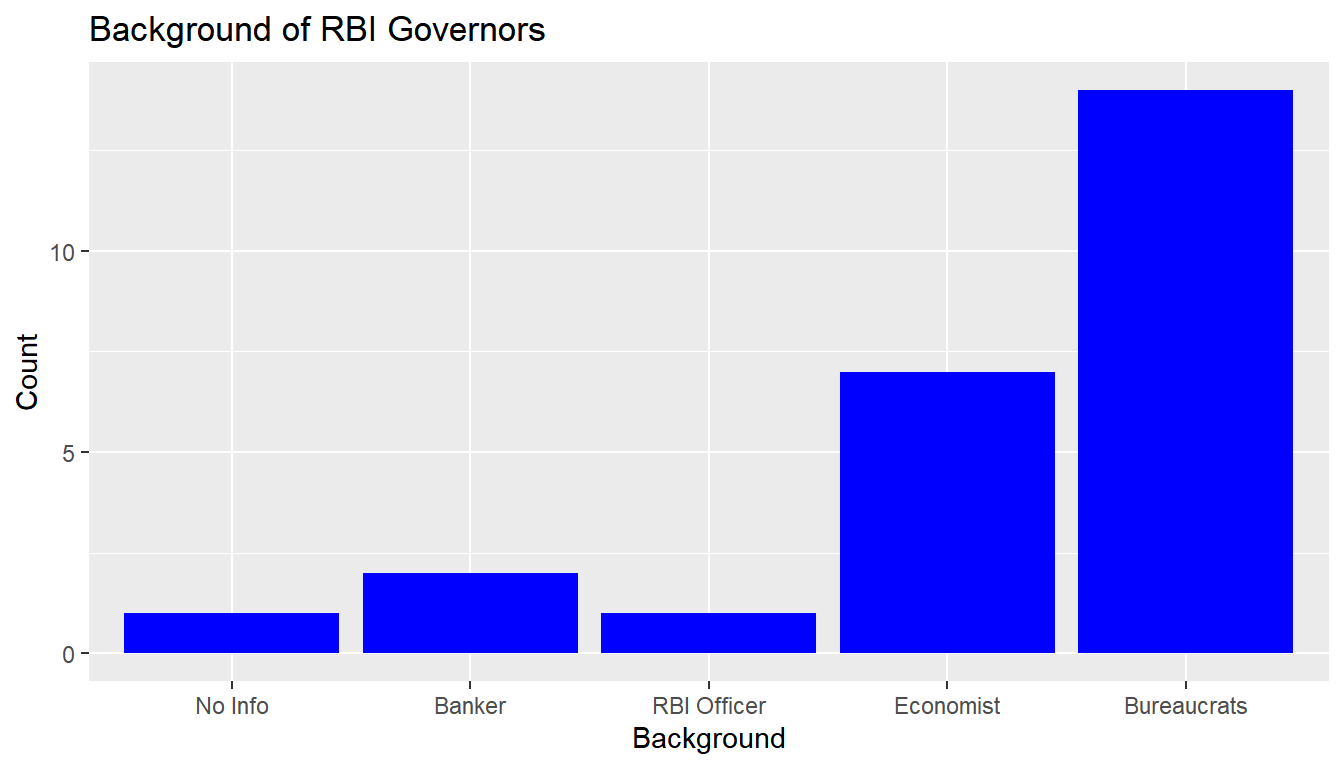
## 4 Economist       7
## 5 Bureaucrats    14
Hmmm.. So there were more bureaucrats than economists.
backgrounds %>%
  ggplot() +
  geom_col(aes(background, count), fill = "blue") +
  xlab("Background") + ylab("Count") +
  ggtitle("Background of RBI Governors")
Summary
-
web scraping is the extraction of data from web sites
-
best for static & well structured HTML pages
-
review robots.txt file
-
HTML code can change any time
-
if API is available, please use it
-
do not overwhelm websites with requests
To get in depth knowledge of R & data science, you can enroll here for our free online R courses.