Preprocessing
This section is optional. You can skip to the Read Data section without any loss of continuity.
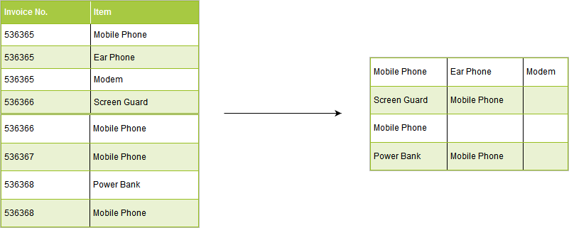
As shown above, the data set has one row per item. We have created a tiny R package mbar,
for data pre-processing. It can be installed from GitHub as shown below:
# install.packages("devtools")
devtools::install_github("rsquaredacademy/mbar")
We will use mbar_prep_data() from the mbar package to reshape the data so that there is one row per transaction with items across columns excluding the column names.
library(mbar)
mba_data     <- read_excel("online-retail.xlsx")
transactions <- mbar_prep_data(mba_data, InvoiceNo, Description)
head(transactions)
## # A tibble: 6 x 1,114
##   item_1 item_2 item_3 item_4 item_5 item_6 item_7 item_8 item_9 item_10 item_11
##   <chr>  <chr>  <chr>  <chr>  <chr>  <chr>  <chr>  <chr>  <chr>  <chr>   <chr>
## 1 WHITE~ "WHIT~ "CREA~ "KNIT~ "RED ~ "SET ~ "GLAS~ ""     ""     ""      ""
## 2 HAND ~ "HAND~ ""     ""     ""     ""     ""     ""     ""     ""      ""
## 3 ASSOR~ "POPP~ "POPP~ "FELT~ "IVOR~ "BOX ~ "BOX ~ "BOX ~ "HOME~ "LOVE ~ "RECIP~
## 4 JAM M~ "RED ~ "YELL~ "BLUE~ ""     ""     ""     ""     ""     ""      ""
## 5 BATH ~ ""     ""     ""     ""     ""     ""     ""     ""     ""      ""
## 6 ALARM~ "ALAR~ "ALAR~ "PAND~ "STAR~ "INFL~ "VINT~ "SET/~ "ROUN~ "SPACE~ "LUNCH~
## # ... with 1,103 more variables: item_12 <chr>, item_13 <chr>, item_14 <chr>,
## #   item_15 <chr>, item_16 <chr>, item_17 <chr>, item_18 <chr>, item_19 <chr>,
## #   item_20 <chr>, item_21 <chr>, item_22 <chr>, item_23 <chr>, item_24 <chr>,
## #   item_25 <chr>, item_26 <chr>, item_27 <chr>, item_28 <chr>, item_29 <chr>,
## #   item_30 <chr>, item_31 <chr>, item_32 <chr>, item_33 <chr>, item_34 <chr>,
## #   item_35 <chr>, item_36 <chr>, item_37 <chr>, item_38 <chr>, item_39 <chr>,
## #   item_40 <chr>, item_41 <chr>, item_42 <chr>, item_43 <chr>, item_44 <chr>,
## #   item_45 <chr>, item_46 <chr>, item_47 <chr>, item_48 <chr>, item_49 <chr>,
## #   item_50 <chr>, item_51 <chr>, item_52 <chr>, item_53 <chr>, item_54 <chr>,
## #   item_55 <chr>, item_56 <chr>, item_57 <chr>, item_58 <chr>, item_59 <chr>,
## #   item_60 <chr>, item_61 <chr>, item_62 <chr>, item_63 <chr>, item_64 <chr>,
## #   item_65 <chr>, item_66 <chr>, item_67 <chr>, item_68 <chr>, item_69 <chr>,
## #   item_70 <chr>, item_71 <chr>, item_72 <chr>, item_73 <chr>, item_74 <chr>,
## #   item_75 <chr>, item_76 <chr>, item_77 <chr>, item_78 <chr>, item_79 <chr>,
## #   item_80 <chr>, item_81 <chr>, item_82 <chr>, item_83 <chr>, item_84 <chr>,
## #   item_85 <chr>, item_86 <chr>, item_87 <chr>, item_88 <chr>, item_89 <chr>,
## #   item_90 <chr>, item_91 <chr>, item_92 <chr>, item_93 <chr>, item_94 <chr>,
## #   item_95 <chr>, item_96 <chr>, item_97 <chr>, item_98 <chr>, item_99 <chr>,
## #   item_100 <chr>, item_101 <chr>, item_102 <chr>, item_103 <chr>,
## #   item_104 <chr>, item_105 <chr>, item_106 <chr>, item_107 <chr>,
## #   item_108 <chr>, item_109 <chr>, item_110 <chr>, item_111 <chr>, ...
Read Data
It is now time to read data into R. We will use read.transactions() from arules package. The data cannot be read using read.csv() or read_csv() owing to the way it is structured. We will read the transaction_data.csv file as it contains the data we had modified in the previous step. We need to specify the following in order to read the data set:
-
name of the data set within quotes (single or double)
-
the format of the data, if each line represnts a transaction, use
basket, and if each line represents an item in the transaction, use single
-
the separator used to separate the items in a transaction
In our data set, each line represents a transaction and the items in the transaction are separated by a ,.
basket_data <- read.transactions("transaction_data.csv", format = "basket",
  sep = ",")
basket_data
## transactions in sparse format with
##  25901 transactions (rows) and
##  10085 items (columns)
The read.transactions() function allows you to read data where each row represents a item and not a transaction. In that case, the format argument should be set to the value single and the cols argument should specify the names or positions of the columns that represent the transaction id and item id. We tried to read data in this way as well but failed to do so. However, the code is available below for other users to try and let us know if you find a way to get it to work or spot any mistakes we may have made.
get_data <- read.transactions("retail.csv",
  format = "single",
  sep = ",",
  cols = c("InvoiceNo", "item"))
We were able to read the data when we removed the sep argument from the above code, but the result from the summary() function was way different than what we see in the next section i.e. it showed higher number of transactions and items.
Item Frequency Plot
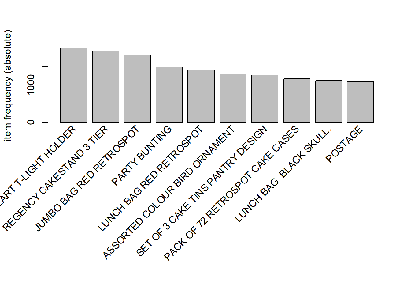
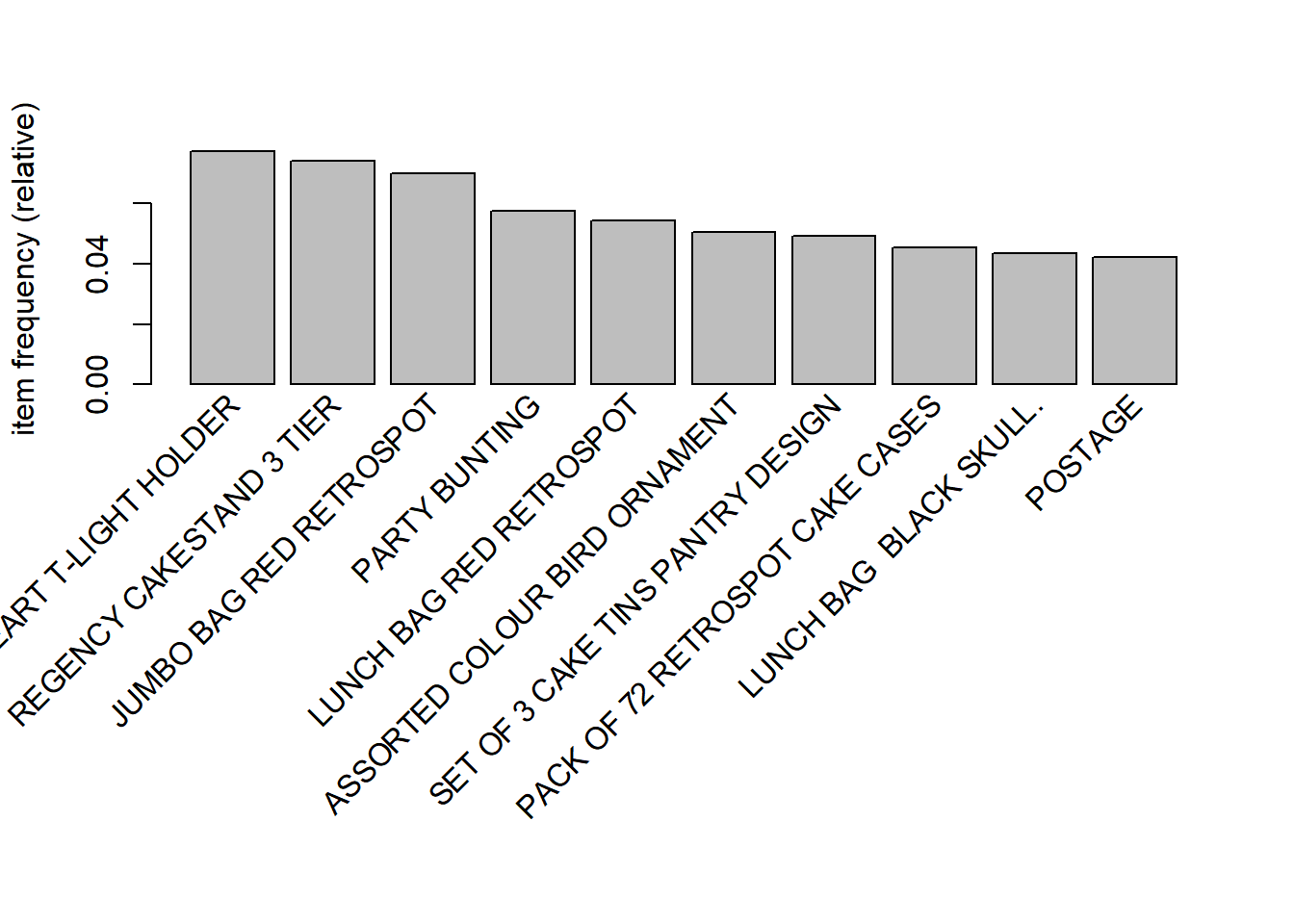
The most frequent items in the data set can be plotted using itemFrequencyPlot(). We can specify the number of items to be plotted and whether the Y axis should represent the absolute or relative number of transactions that include the item.
The topN argument can be used to specify the number of items to be plotted and the type argument can be used to specify whether the Y axis represents absolute/relative frequency of the items.
itemFrequencyPlot(basket_data, topN = 10, type = 'absolute')
In the below plot, the Y axis represents the relative frequency of the items plotted.
itemFrequencyPlot(basket_data, topN = 10, type = 'relative')

Generate Rules
Finally, to the part you all have been waiting for, rules generation. The apriori() function is used for generating the rules. We will first learn the different inputs that must be specified and later on play around with them and see how the rules generated change.
The first input is the data set, which in our case is basket_data. Next, we will supply the mining parameters using the parameter argument:
-
supp: minimum support for an itemset
-
conf: minimum confidence
-
maxlen: maximum number of items the antecedent may include
-
target: the type of association mined i.e. rules
The parameter argument takes several additional inputs but to get started, it is sufficient to know those mentioned above. All the inputs are supplied using a list().
For our case study, we will specify the following:
-
support: 0.009
-
confidence: 0.8
-
maxlen: 4
Keep in mind, mining association rules with very low values for support will result in a large number of rules being generated, resulting in long execution time and the process will eventually run out of memory.
rules <- apriori(basket_data, parameter = list(supp=0.009, conf=0.8,
    target = "rules", maxlen = 4))
## Apriori
##
## Parameter specification:
##  confidence minval smax arem  aval originalSupport maxtime support minlen
##         0.8    0.1    1 none FALSE            TRUE       5   0.009      1
##  maxlen target  ext
##       4  rules TRUE
##
## Algorithmic control:
##  filter tree heap memopt load sort verbose
##     0.1 TRUE TRUE  FALSE TRUE    2    TRUE
##
## Absolute minimum support count: 233
##
## set item appearances ...[0 item(s)] done [0.00s].
## set transactions ...[10085 item(s), 25901 transaction(s)] done [1.08s].
## sorting and recoding items ... [508 item(s)] done [0.02s].
## creating transaction tree ... done [0.06s].
## checking subsets of size 1 2 3 4
## Warning in apriori(basket_data, parameter = list(supp = 0.009, conf = 0.8, :
## Mining stopped (maxlen reached). Only patterns up to a length of 4 returned!
##  done [0.07s].
## writing ... [22 rule(s)] done [0.00s].
## creating S4 object  ... done [0.02s].
Change the values of supp, conf and maxlen, and observe how the rules generated change.
Rules Summary
Once the rules have been generated by apriori(), we can use summary() to get some basic information such as rule length distribution.
summary(rules)
## set of 22 rules
##
## rule length distribution (lhs + rhs):sizes
##  2  3  4
## 11  9  2
##
##    Min. 1st Qu.  Median    Mean 3rd Qu.    Max.
##   2.000   2.000   2.500   2.591   3.000   4.000
##
## summary of quality measures:
##     support           confidence        coverage             lift
##  Min.   :0.009034   Min.   :0.8035   Min.   :0.009614   Min.   :22.59
##  1st Qu.:0.010453   1st Qu.:0.8530   1st Qu.:0.011592   1st Qu.:25.02
##  Median :0.013223   Median :0.8868   Median :0.014362   Median :55.94
##  Mean   :0.012760   Mean   :0.9120   Mean   :0.014061   Mean   :48.55
##  3rd Qu.:0.014362   3rd Qu.:1.0000   3rd Qu.:0.014362   3rd Qu.:61.23
##  Max.   :0.018339   Max.   :1.0000   Max.   :0.021544   Max.   :71.30
##      count
##  Min.   :234.0
##  1st Qu.:270.8
##  Median :342.5
##  Mean   :330.5
##  3rd Qu.:372.0
##  Max.   :475.0
##
## mining info:
##         data ntransactions support confidence
##  basket_data         25901   0.009        0.8
The output from summary() does not display the rules though. To view the rules, we have to use inspect().
Inspect Rules
The inspect() function will display the rules along with:
-
support
-
confidence
-
lift
-
count
Before you inspect the rules, you can sort it by support, confidence or lift. In the below, output, we sort the rules by confidence in descending order before inspecting them.
basket_rules <- sort(rules, by = 'confidence', decreasing = TRUE)
inspect(basket_rules[1:10])
##      lhs                                  rhs                                   support confidence    coverage     lift count
## [1]  {BACK DOOR}                       => {KEY FOB}                         0.009613528  1.0000000 0.009613528 61.23168   249
## [2]  {SET 3 RETROSPOT TEA}             => {SUGAR}                           0.014362380  1.0000000 0.014362380 69.62634   372
## [3]  {SUGAR}                           => {SET 3 RETROSPOT TEA}             0.014362380  1.0000000 0.014362380 69.62634   372
## [4]  {SET 3 RETROSPOT TEA}             => {COFFEE}                          0.014362380  1.0000000 0.014362380 55.94168   372
## [5]  {SUGAR}                           => {COFFEE}                          0.014362380  1.0000000 0.014362380 55.94168   372
## [6]  {SHED}                            => {KEY FOB}                         0.011273696  1.0000000 0.011273696 61.23168   292
## [7]  {SET 3 RETROSPOT TEA,
##       SUGAR}                           => {COFFEE}                          0.014362380  1.0000000 0.014362380 55.94168   372
## [8]  {COFFEE,
##       SET 3 RETROSPOT TEA}             => {SUGAR}                           0.014362380  1.0000000 0.014362380 69.62634   372
## [9]  {COFFEE,
##       SUGAR}                           => {SET 3 RETROSPOT TEA}             0.014362380  1.0000000 0.014362380 69.62634   372
## [10] {PINK REGENCY TEACUP AND SAUCER,
##       REGENCY CAKESTAND 3 TIER,
##       ROSES REGENCY TEACUP AND SAUCER} => {GREEN REGENCY TEACUP AND SAUCER} 0.009999614  0.8900344 0.011235087 25.16679   259
Redundant & Non Redundant Rules
Redundant Rules
A rule is redundant if a more general rules with the same or a higher confidence exists. That is, a more specific rule is redundant if it is only equally or even less predictive than a more general rule. A rule is more general if it has the same RHS but one or more items removed from the LHS.
Example 1
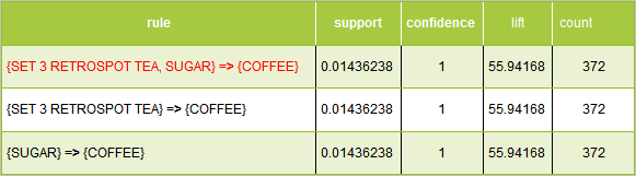
In the above example, the first rule has the same support, condifence and lift as the next two rules. The second item in the left hand side of the rule is not adding any value and as such makes the rule redundant.
Example 2
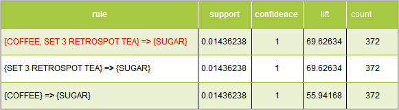
In the above example, the first two rules have the same support, condifence and lift. The third rule differs only with respect to lift.
Example 3
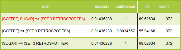
In the above example, the first and third rule have the same support, condifence and lift. The second rule is different with respect to confidence and lift.
Now that we have understood what redundant rules are and how to identify them, let us use the below R code to inspect them.
inspect(rules[is.redundant(rules)])
##     lhs                             rhs                   support    confidence
## [1] {SET 3 RETROSPOT TEA,SUGAR}  => {COFFEE}              0.01436238 1
## [2] {COFFEE,SET 3 RETROSPOT TEA} => {SUGAR}               0.01436238 1
## [3] {COFFEE,SUGAR}               => {SET 3 RETROSPOT TEA} 0.01436238 1
##     coverage   lift     count
## [1] 0.01436238 55.94168 372
## [2] 0.01436238 69.62634 372
## [3] 0.01436238 69.62634 372
Non-redundant Rules
Now let us look at the non-redundant rules.
inspect(rules[!is.redundant(rules)])
##      lhs                                     rhs                                   support confidence    coverage     lift count
## [1]  {REGENCY TEA PLATE PINK}             => {REGENCY TEA PLATE GREEN}         0.009034400  0.8863636 0.010192657 71.29722   234
## [2]  {BACK DOOR}                          => {KEY FOB}                         0.009613528  1.0000000 0.009613528 61.23168   249
## [3]  {SET 3 RETROSPOT TEA}                => {SUGAR}                           0.014362380  1.0000000 0.014362380 69.62634   372
## [4]  {SUGAR}                              => {SET 3 RETROSPOT TEA}             0.014362380  1.0000000 0.014362380 69.62634   372
## [5]  {SET 3 RETROSPOT TEA}                => {COFFEE}                          0.014362380  1.0000000 0.014362380 55.94168   372
## [6]  {COFFEE}                             => {SET 3 RETROSPOT TEA}             0.014362380  0.8034557 0.017875758 55.94168   372
## [7]  {SUGAR}                              => {COFFEE}                          0.014362380  1.0000000 0.014362380 55.94168   372
## [8]  {COFFEE}                             => {SUGAR}                           0.014362380  0.8034557 0.017875758 55.94168   372
## [9]  {REGENCY TEA PLATE GREEN}            => {REGENCY TEA PLATE ROSES}         0.010347091  0.8322981 0.012431952 55.99313   268
## [10] {SHED}                               => {KEY FOB}                         0.011273696  1.0000000 0.011273696 61.23168   292
## [11] {SET/6 RED SPOTTY PAPER CUPS}        => {SET/6 RED SPOTTY PAPER PLATES}   0.012084476  0.8087855 0.014941508 44.38211   313
## [12] {SET/20 RED RETROSPOT PAPER NAPKINS,
##       SET/6 RED SPOTTY PAPER CUPS}        => {SET/6 RED SPOTTY PAPER PLATES}   0.009111617  0.8872180 0.010269874 48.68609   236
## [13] {PINK REGENCY TEACUP AND SAUCER,
##       ROSES REGENCY TEACUP AND SAUCER}    => {GREEN REGENCY TEACUP AND SAUCER} 0.018339060  0.8828996 0.020771399 24.96505   475
## [14] {GREEN REGENCY TEACUP AND SAUCER,
##       PINK REGENCY TEACUP AND SAUCER}     => {ROSES REGENCY TEACUP AND SAUCER} 0.018339060  0.8512545 0.021543570 22.59051   475
## [15] {PINK REGENCY TEACUP AND SAUCER,
##       REGENCY CAKESTAND 3 TIER}           => {ROSES REGENCY TEACUP AND SAUCER} 0.011235087  0.8584071 0.013088298 22.78033   291
## [16] {PINK REGENCY TEACUP AND SAUCER,
##       REGENCY CAKESTAND 3 TIER}           => {GREEN REGENCY TEACUP AND SAUCER} 0.011312305  0.8643068 0.013088298 24.43931   293
## [17] {STRAWBERRY CHARLOTTE BAG,
##       WOODLAND CHARLOTTE BAG}             => {RED RETROSPOT CHARLOTTE BAG}     0.010771785  0.8110465 0.013281340 23.65644   279
## [18] {PINK REGENCY TEACUP AND SAUCER,
##       REGENCY CAKESTAND 3 TIER,
##       ROSES REGENCY TEACUP AND SAUCER}    => {GREEN REGENCY TEACUP AND SAUCER} 0.009999614  0.8900344 0.011235087 25.16679   259
## [19] {GREEN REGENCY TEACUP AND SAUCER,
##       PINK REGENCY TEACUP AND SAUCER,
##       REGENCY CAKESTAND 3 TIER}           => {ROSES REGENCY TEACUP AND SAUCER} 0.009999614  0.8839590 0.011312305 23.45843   259
What influenced purchase of product X?
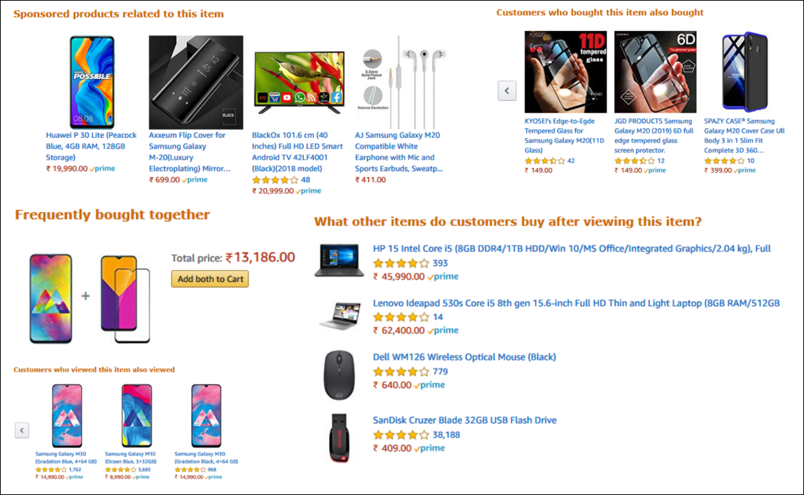
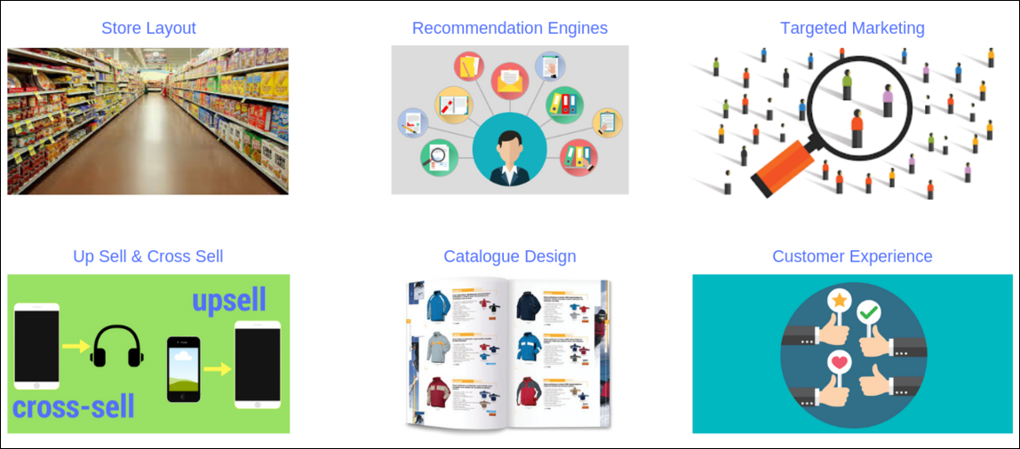
So far, we have learnt how to generate, inspect and prune rules. Now, how do we use these rules? To make business sense, we need to come up with a set of rules that can be used either for product placement in physical stores or as recommendations in an online store or for targeted marketing via email campaigns etc. To achieve that, we need to know 2 things:
-
what products influenced the purchase of product X?
-
what purchases did product X influence?
For our case study, we can modify the above questions as:
What influenced the purchase of sugar?
To view the products which influenced the purchase of sugar, we will continue to use the apriori() function but add one more argument, appearance. It restricts the appearance of the items. Since we want the right hand side of the rules to have only one value, sugar, we will set the rhs argument to sugar. The left hand side of the rules should include all the products that influenced the purchase of sugar i.e. it will exclude sugar. We will use the default argument and supply it the value lhs i.e. all items excluding sugar can appear on the left hand side of the rule by default.
sugar_rules <- apriori(basket_data, parameter = list(supp = 0.009, conf = 0.8),
  appearance = list(default = "lhs", rhs = "SUGAR"))
## Apriori
##
## Parameter specification:
##  confidence minval smax arem  aval originalSupport maxtime support minlen
##         0.8    0.1    1 none FALSE            TRUE       5   0.009      1
##  maxlen target  ext
##      10  rules TRUE
##
## Algorithmic control:
##  filter tree heap memopt load sort verbose
##     0.1 TRUE TRUE  FALSE TRUE    2    TRUE
##
## Absolute minimum support count: 233
##
## set item appearances ...[1 item(s)] done [0.00s].
## set transactions ...[10085 item(s), 25901 transaction(s)] done [0.86s].
## sorting and recoding items ... [508 item(s)] done [0.02s].
## creating transaction tree ... done [0.04s].
## checking subsets of size 1 2 3 4 done [0.07s].
## writing ... [3 rule(s)] done [0.00s].
## creating S4 object  ... done [0.02s].
rules_sugar <- sort(sugar_rules, by = "confidence", decreasing = TRUE)
inspect(rules_sugar)
##     lhs                             rhs     support    confidence coverage
## [1] {SET 3 RETROSPOT TEA}        => {SUGAR} 0.01436238 1.0000000  0.01436238
## [2] {COFFEE,SET 3 RETROSPOT TEA} => {SUGAR} 0.01436238 1.0000000  0.01436238
## [3] {COFFEE}                     => {SUGAR} 0.01436238 0.8034557  0.01787576
##     lift     count
## [1] 69.62634 372
## [2] 69.62634 372
## [3] 55.94168 372
For the support and confidence we have mentioned, we know the following products influenced the purchase of sugar:
-
COFFEE
-
SET 3 RETROSPOT TEA
What purchases did product X influence?
Now that we know what products influenced the purchase of sugar, let us answer the second question.
What purchases did sugar influence?
In this case, we want sugar to be on the left hand side of the rule and all the products it influenced to be on the right hand side. We set the lhs argument to sugar and the default argument to rhs as all the products, the purchase of which was influenced by sugar should appear on the left hand side of the rule by default.
sugar_rules <- apriori(basket_data, parameter = list(supp = 0.009, conf = 0.8),
  appearance = list(default = "rhs", lhs = "SUGAR"))
## Apriori
##
## Parameter specification:
##  confidence minval smax arem  aval originalSupport maxtime support minlen
##         0.8    0.1    1 none FALSE            TRUE       5   0.009      1
##  maxlen target  ext
##      10  rules TRUE
##
## Algorithmic control:
##  filter tree heap memopt load sort verbose
##     0.1 TRUE TRUE  FALSE TRUE    2    TRUE
##
## Absolute minimum support count: 233
##
## set item appearances ...[1 item(s)] done [0.00s].
## set transactions ...[10085 item(s), 25901 transaction(s)] done [0.76s].
## sorting and recoding items ... [508 item(s)] done [0.02s].
## creating transaction tree ... done [0.03s].
## checking subsets of size 1 2 done [0.01s].
## writing ... [2 rule(s)] done [0.00s].
## creating S4 object  ... done [0.01s].
rules_sugar <- sort(sugar_rules, by = "confidence", decreasing = TRUE)
inspect(rules_sugar)
##     lhs        rhs                   support    confidence coverage   lift
## [1] {SUGAR} => {SET 3 RETROSPOT TEA} 0.01436238 1          0.01436238 69.62634
## [2] {SUGAR} => {COFFEE}              0.01436238 1          0.01436238 55.94168
##     count
## [1] 372
## [2] 372
For the support and confidence we have mentioned, we know the purchase of the following products were influenced by sugar:
-
COFFEE
-
SET 3 RETROSPOT TEA
Top Rules
Let us take a look at the top rules by
Support
supp_rules <- sort(rules, by = 'support', decreasing = TRUE)
top_rules <- supp_rules[1:10]
inspect(top_rules)
##      lhs                                  rhs                                  support confidence   coverage     lift count
## [1]  {PINK REGENCY TEACUP AND SAUCER,
##       ROSES REGENCY TEACUP AND SAUCER} => {GREEN REGENCY TEACUP AND SAUCER} 0.01833906  0.8828996 0.02077140 24.96505   475
## [2]  {GREEN REGENCY TEACUP AND SAUCER,
##       PINK REGENCY TEACUP AND SAUCER}  => {ROSES REGENCY TEACUP AND SAUCER} 0.01833906  0.8512545 0.02154357 22.59051   475
## [3]  {SET 3 RETROSPOT TEA}             => {SUGAR}                           0.01436238  1.0000000 0.01436238 69.62634   372
## [4]  {SUGAR}                           => {SET 3 RETROSPOT TEA}             0.01436238  1.0000000 0.01436238 69.62634   372
## [5]  {SET 3 RETROSPOT TEA}             => {COFFEE}                          0.01436238  1.0000000 0.01436238 55.94168   372
## [6]  {COFFEE}                          => {SET 3 RETROSPOT TEA}             0.01436238  0.8034557 0.01787576 55.94168   372
## [7]  {SUGAR}                           => {COFFEE}                          0.01436238  1.0000000 0.01436238 55.94168   372
## [8]  {COFFEE}                          => {SUGAR}                           0.01436238  0.8034557 0.01787576 55.94168   372
## [9]  {SET 3 RETROSPOT TEA,
##       SUGAR}                           => {COFFEE}                          0.01436238  1.0000000 0.01436238 55.94168   372
## [10] {COFFEE,
##       SET 3 RETROSPOT TEA}             => {SUGAR}                           0.01436238  1.0000000 0.01436238 69.62634   372
Confidence
conf_rules <- sort(rules, by = 'confidence', decreasing = TRUE)
top_rules <- conf_rules[1:10]
inspect(top_rules)
##      lhs                                  rhs                                   support confidence    coverage     lift count
## [1]  {BACK DOOR}                       => {KEY FOB}                         0.009613528  1.0000000 0.009613528 61.23168   249
## [2]  {SET 3 RETROSPOT TEA}             => {SUGAR}                           0.014362380  1.0000000 0.014362380 69.62634   372
## [3]  {SUGAR}                           => {SET 3 RETROSPOT TEA}             0.014362380  1.0000000 0.014362380 69.62634   372
## [4]  {SET 3 RETROSPOT TEA}             => {COFFEE}                          0.014362380  1.0000000 0.014362380 55.94168   372
## [5]  {SUGAR}                           => {COFFEE}                          0.014362380  1.0000000 0.014362380 55.94168   372
## [6]  {SHED}                            => {KEY FOB}                         0.011273696  1.0000000 0.011273696 61.23168   292
## [7]  {SET 3 RETROSPOT TEA,
##       SUGAR}                           => {COFFEE}                          0.014362380  1.0000000 0.014362380 55.94168   372
## [8]  {COFFEE,
##       SET 3 RETROSPOT TEA}             => {SUGAR}                           0.014362380  1.0000000 0.014362380 69.62634   372
## [9]  {COFFEE,
##       SUGAR}                           => {SET 3 RETROSPOT TEA}             0.014362380  1.0000000 0.014362380 69.62634   372
## [10] {PINK REGENCY TEACUP AND SAUCER,
##       REGENCY CAKESTAND 3 TIER,
##       ROSES REGENCY TEACUP AND SAUCER} => {GREEN REGENCY TEACUP AND SAUCER} 0.009999614  0.8900344 0.011235087 25.16679   259
Lift
lift_rules <- sort(rules, by = 'lift', decreasing = TRUE)
top_rules <- lift_rules[1:10]
inspect(top_rules)
##      lhs                             rhs                       support
## [1]  {REGENCY TEA PLATE PINK}     => {REGENCY TEA PLATE GREEN} 0.009034400
## [2]  {SET 3 RETROSPOT TEA}        => {SUGAR}                   0.014362380
## [3]  {SUGAR}                      => {SET 3 RETROSPOT TEA}     0.014362380
## [4]  {COFFEE,SET 3 RETROSPOT TEA} => {SUGAR}                   0.014362380
## [5]  {COFFEE,SUGAR}               => {SET 3 RETROSPOT TEA}     0.014362380
## [6]  {BACK DOOR}                  => {KEY FOB}                 0.009613528
## [7]  {SHED}                       => {KEY FOB}                 0.011273696
## [8]  {REGENCY TEA PLATE GREEN}    => {REGENCY TEA PLATE ROSES} 0.010347091
## [9]  {SET 3 RETROSPOT TEA}        => {COFFEE}                  0.014362380
## [10] {COFFEE}                     => {SET 3 RETROSPOT TEA}     0.014362380
##      confidence coverage    lift     count
## [1]  0.8863636  0.010192657 71.29722 234
## [2]  1.0000000  0.014362380 69.62634 372
## [3]  1.0000000  0.014362380 69.62634 372
## [4]  1.0000000  0.014362380 69.62634 372
## [5]  1.0000000  0.014362380 69.62634 372
## [6]  1.0000000  0.009613528 61.23168 249
## [7]  1.0000000  0.011273696 61.23168 292
## [8]  0.8322981  0.012431952 55.99313 268
## [9]  1.0000000  0.014362380 55.94168 372
## [10] 0.8034557  0.017875758 55.94168 372

Visualization
To visualize the rules, the authors of arules have created a companion package, arulesViz. It offers several options for visualizing the rules generated by apriori().
Scatter Plot
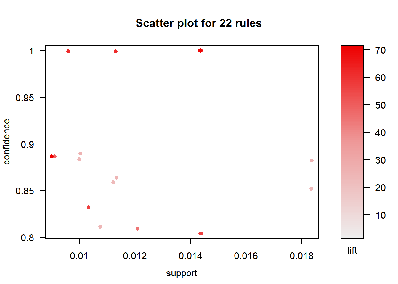
We can use the default plot() method to create a scatter plot. It will plot the support on the X axis, the confidence on the Y axis and the lift is represented by the opaqueness/alpha of the color of the points.
plot(basket_rules)
Network Plot
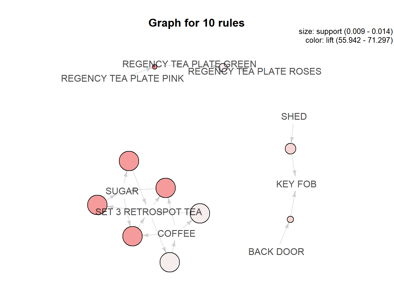
We can create a network plot using the method argument and supplying it the value graph. You can see the directionality of the rule in the below plot. For example, people who buy shed also buy key fob and similarly, people who buy back door also buy key fob. It will be difficult to identify the directionality of the rules when we are trying to plot too many rules. The method argument takes several other values as well.
plot(top_rules, method = 'graph')
Things to keep in mind..
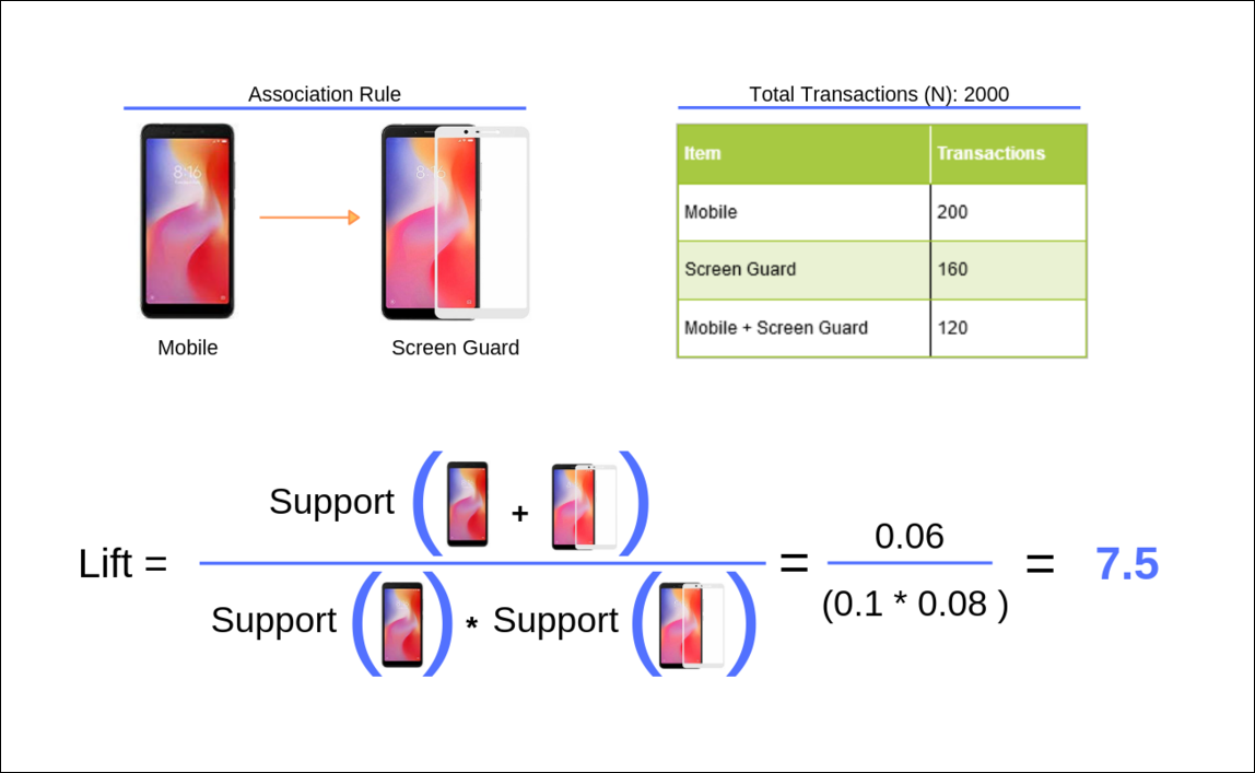
Directionality of rule is lost while using lift
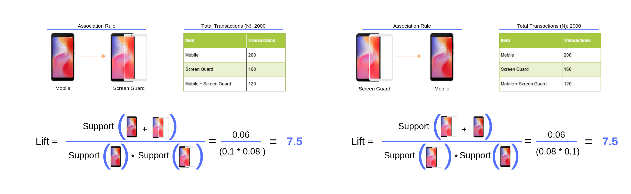
The directionality of a rule is lost while using lift. In the below example, the lift is same for both the following rules:
-
{Mobile Phone} => {Screen Guard}
-
{Screen Guard} => {Mobile Phone}
It is clear that the lift is the same irrespective of the direction of the rule.
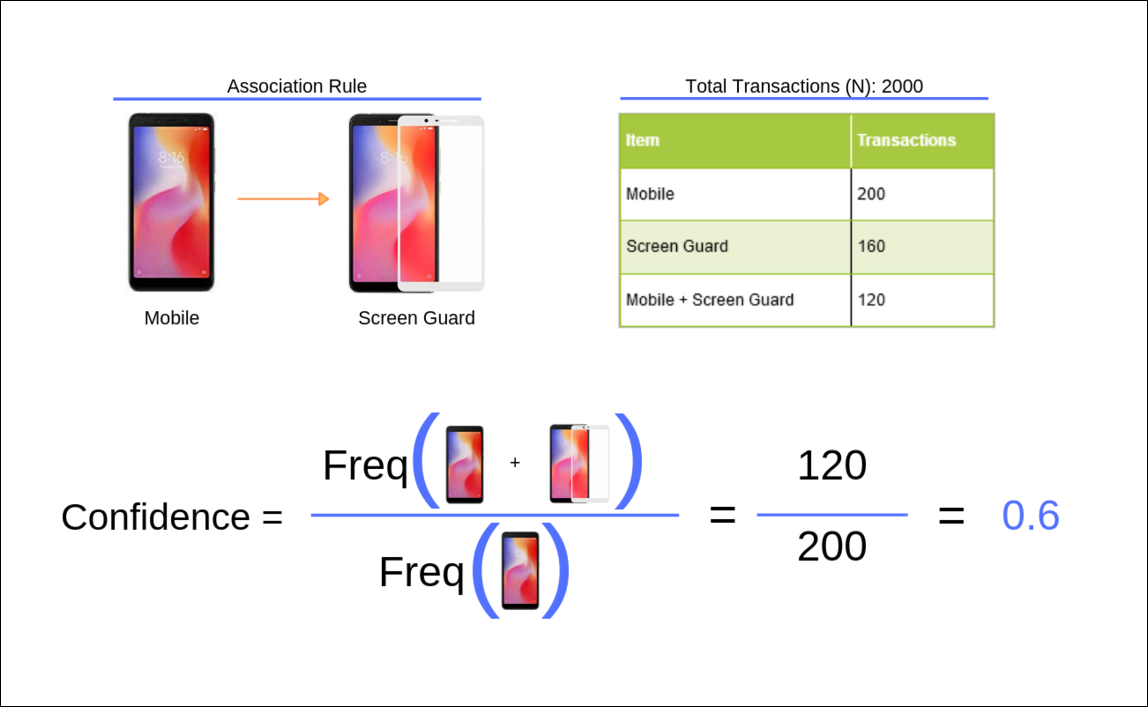
Confidence as a measure can be misleading
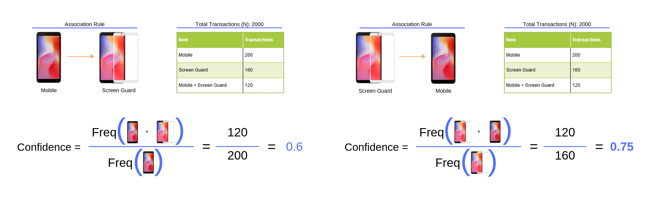
If you look at the below example, the confidence for the second rule, {Screen Guard} => {Mobile Phone}, is greater than the first rule, {Mobile Phone} => {Screen Guard}. It does not mean that we can recommend a mobile phone to a customer who is purchasing a screen guard. It is important to ensure that we do not use rules just because they have high confidence associated with them.
Summary
-
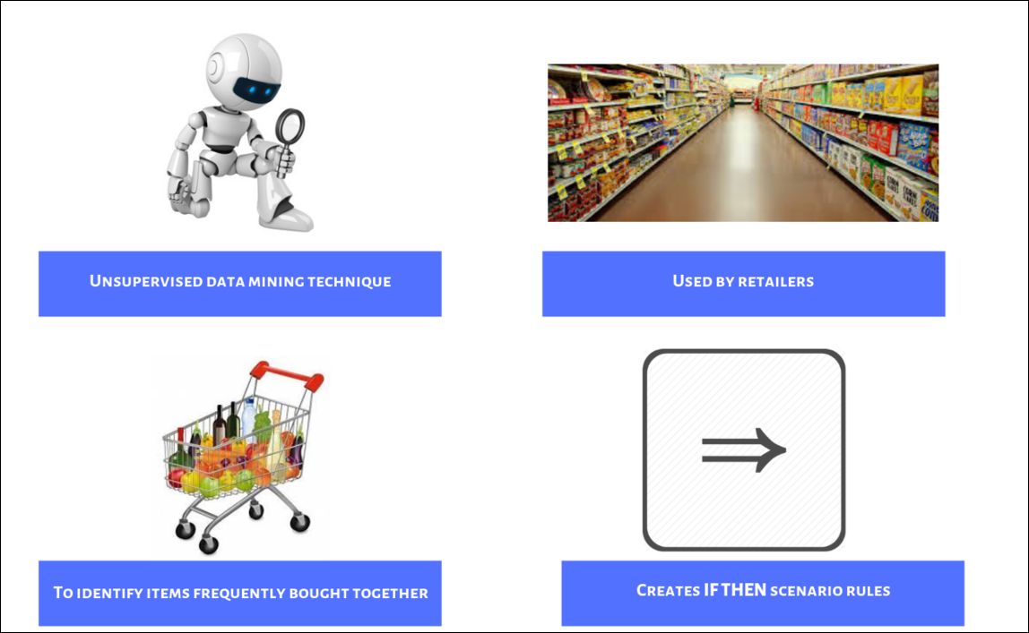
market basket analysis is an unsupervised data mining technique
-
uncovers products frequently bought together
-
creates if-then scenario rules
-
cost-effective, insightful and actionable
-
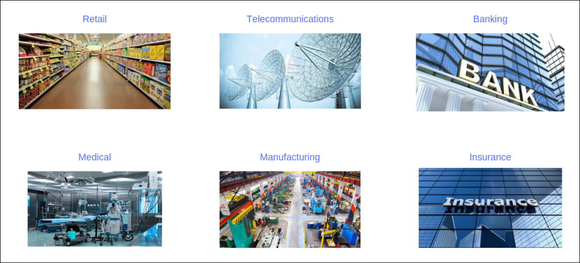
association rule mining has applications in several industries
-
directionality of rule is lost while using lift
-
confidence as a measure can be misleading
Your knowledge of the domain/business matters a lot when you are trying to use market basket analysis. Especially, when you are trying to select or shortlist rules and use them for product placement in a store or for recommending products online. It is a good practice to critically review the rules before implementing them.