Data Visualization with R - Histogram
Introduction
This is the seventh post in the series Data Visualization With R. In the previous post, we learnt about box and whisker plots. In this post, we will learn to:
- create a bare bones histogram
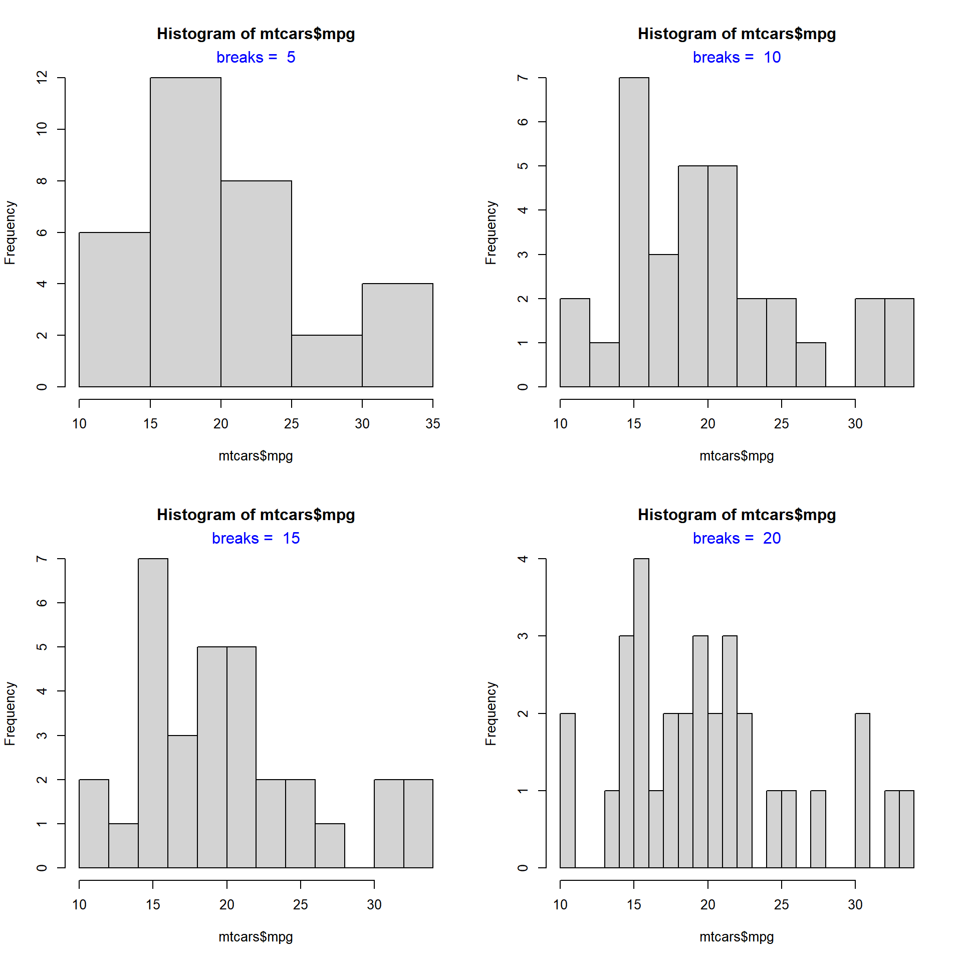
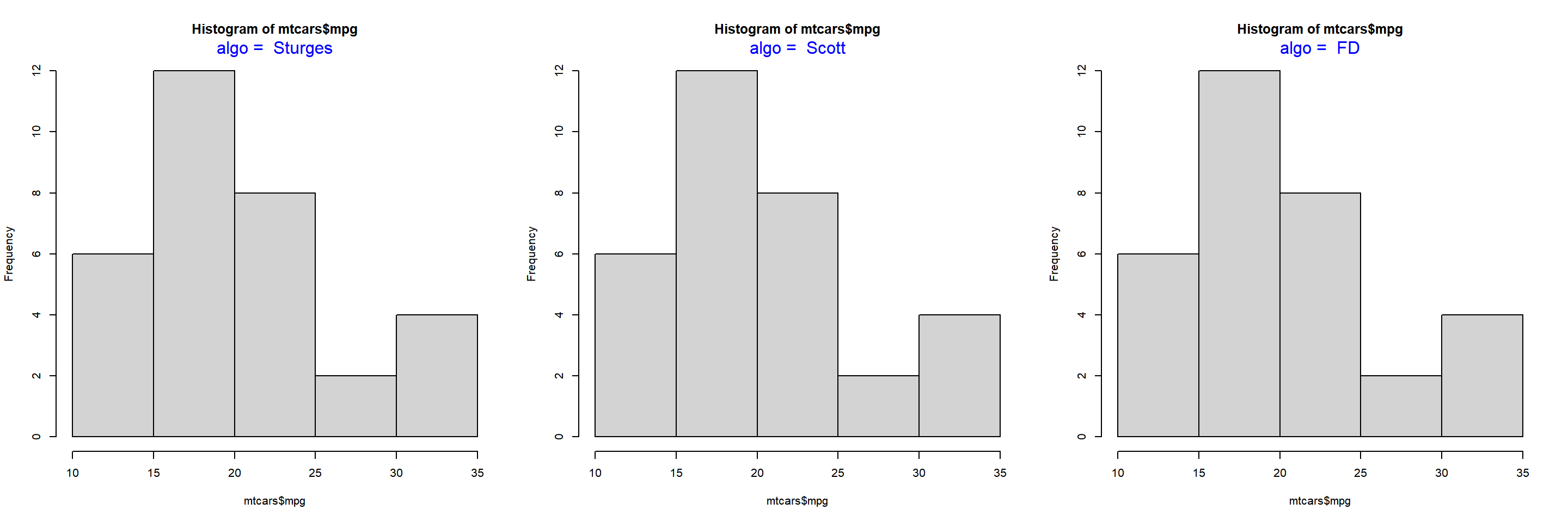
- specify the number of bins/intervals
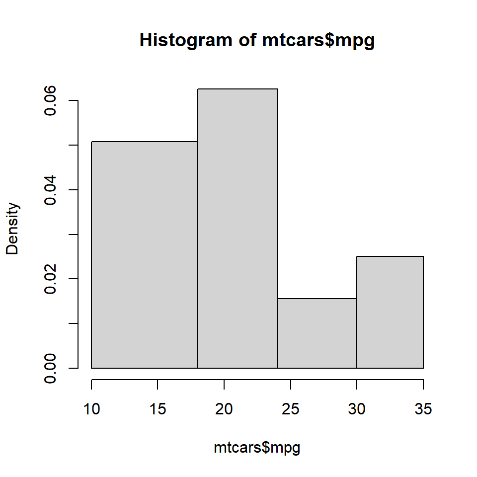
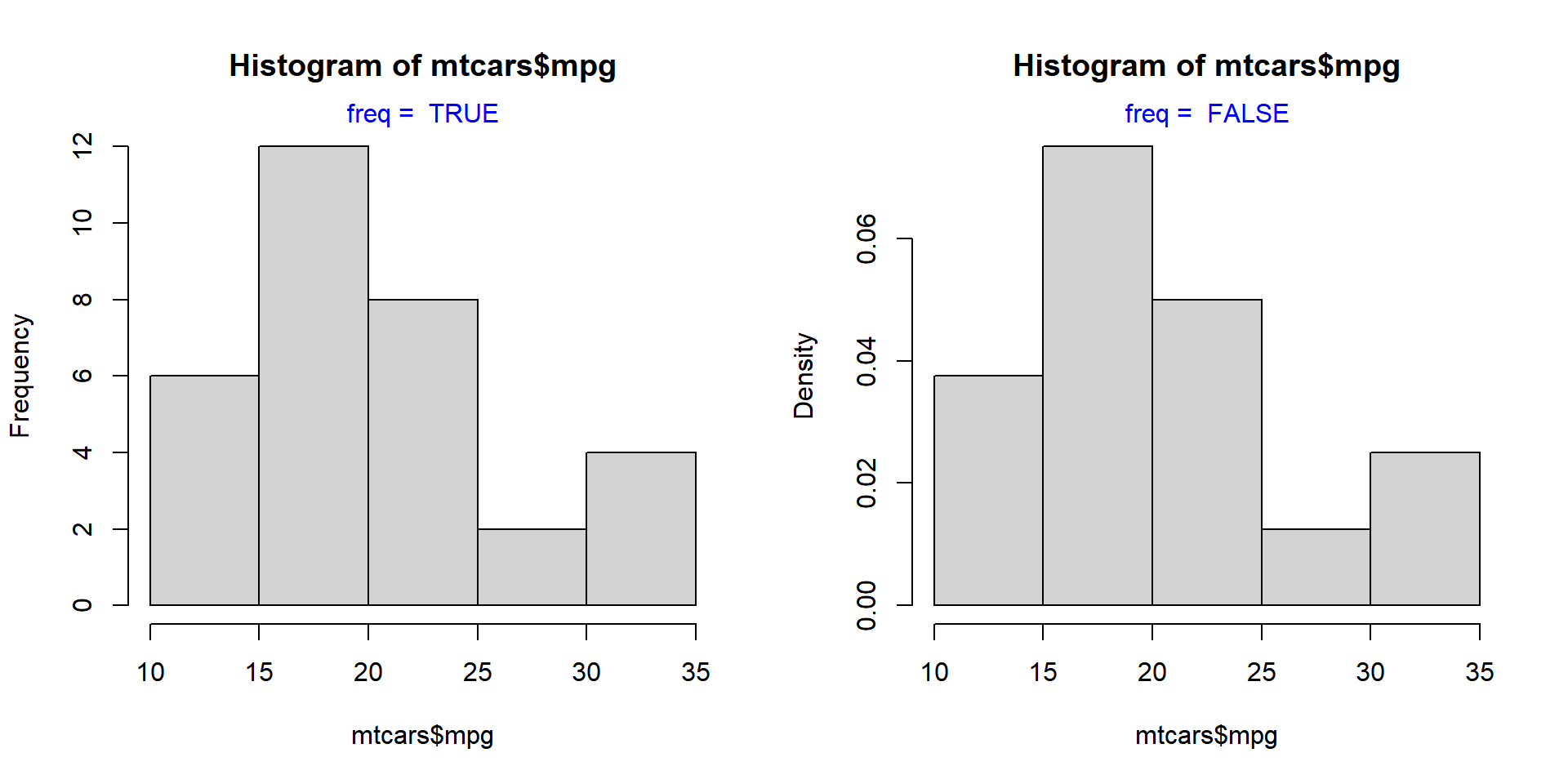
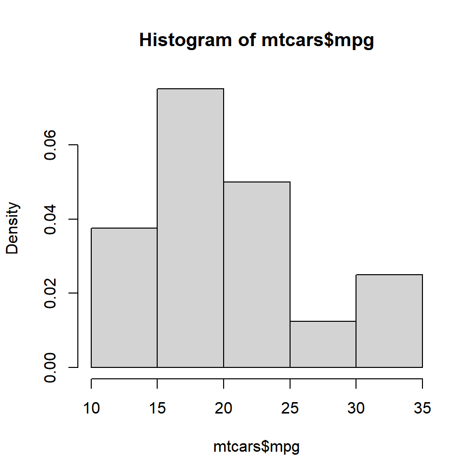
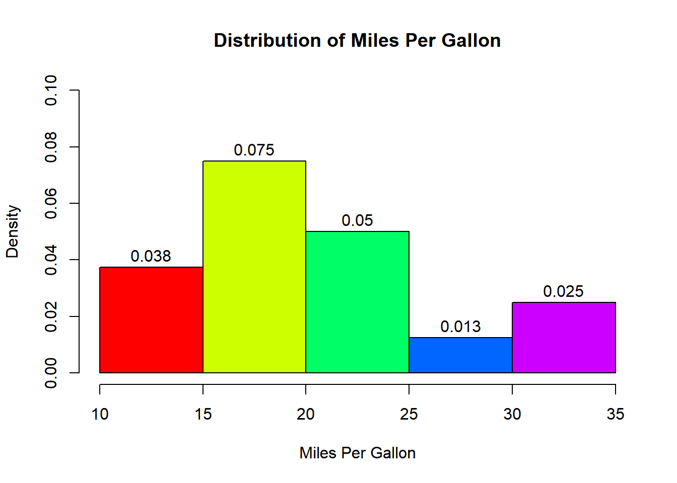
- represent frequency density on the Y axis
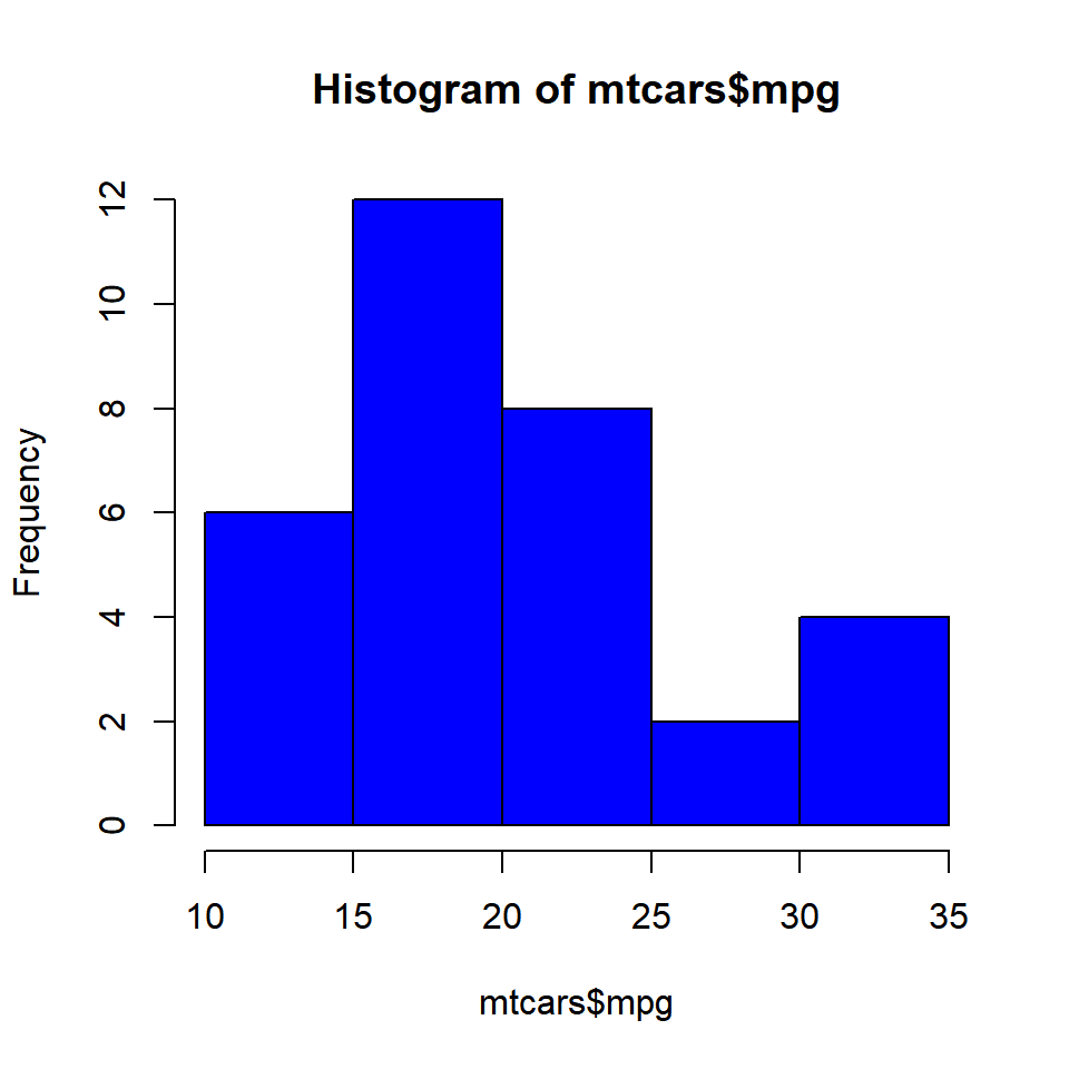
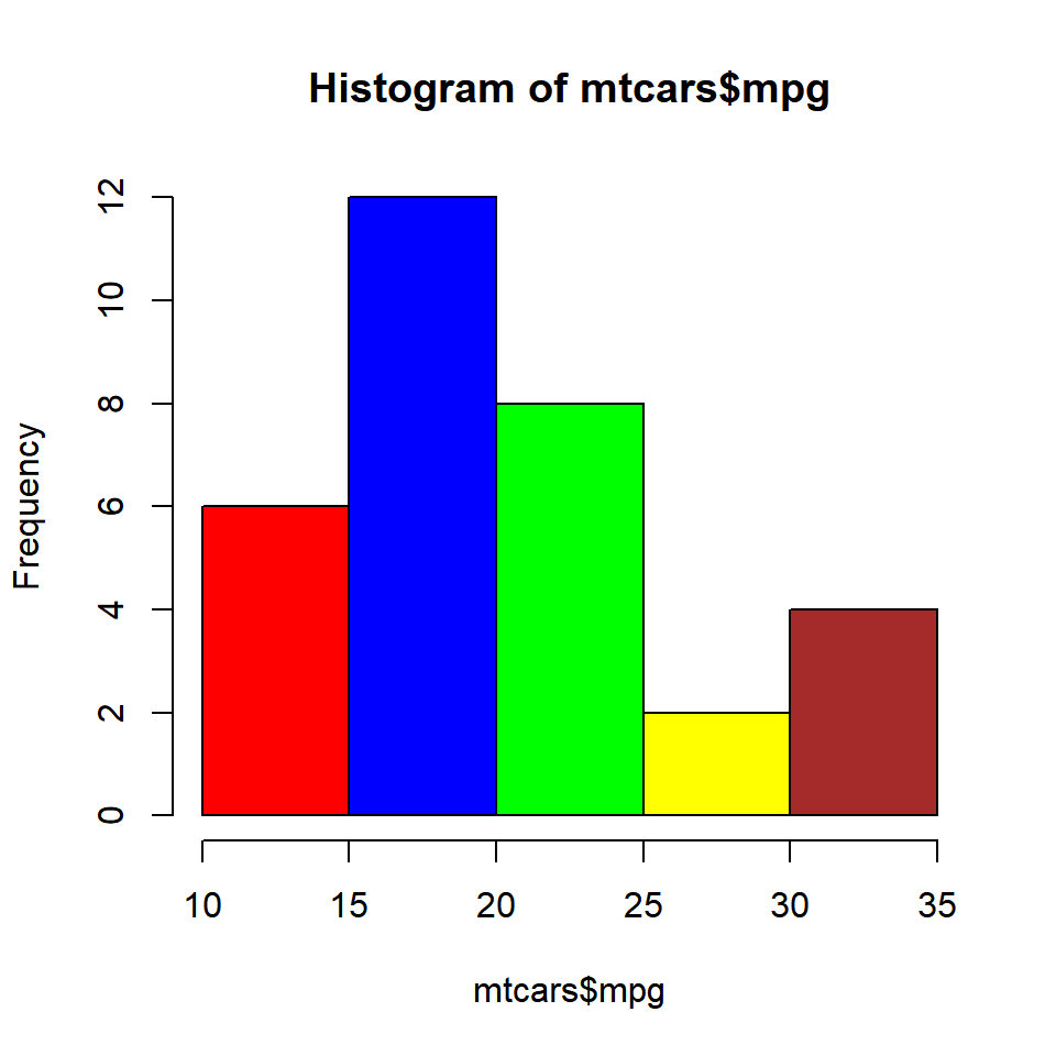
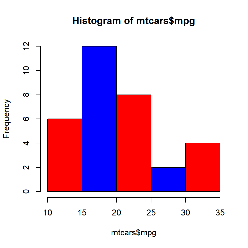
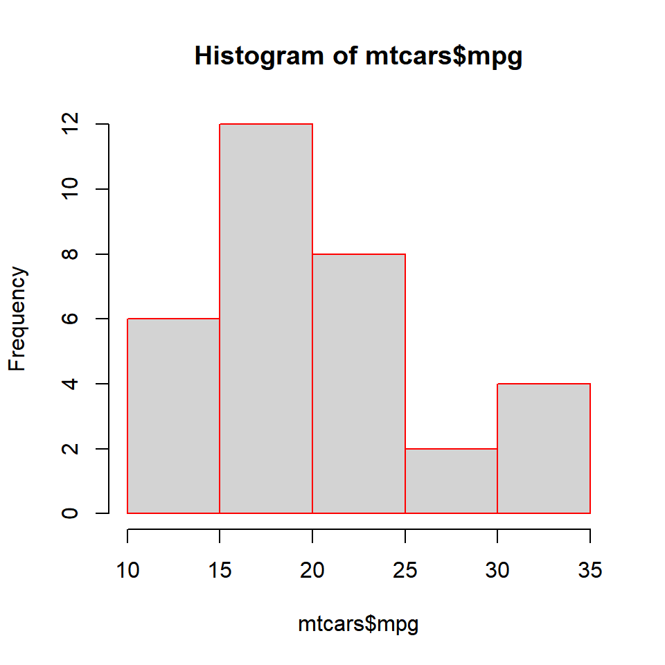
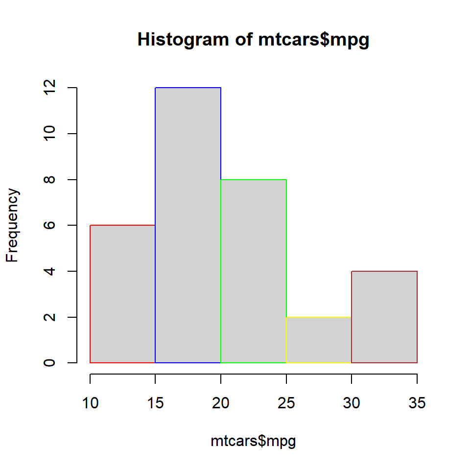
- add colors to the bars and the border
- add labels to the bars
A histogram is a plot that can be used to examine the shape and spread of continuous data. It looks very similar to a bar graph and can be used to detect outliers and skewness in data. The histogram graphically shows the following:
- center (location) of the data
- spread (dispersion) of the data
- skewness
- outliers
- presence of multiple modes
To construct a histogram, the data is split into intervals called bins. The intervals may or may not be equal sized. For each bin, the number of data points that fall into it are counted (frequency). The Y axis of the histogram represents the frequency and the X axis represents the variable.
Libraries, Code & Data
All the data sets used in this post can be found here and code can be downloaded from here.
Distributions
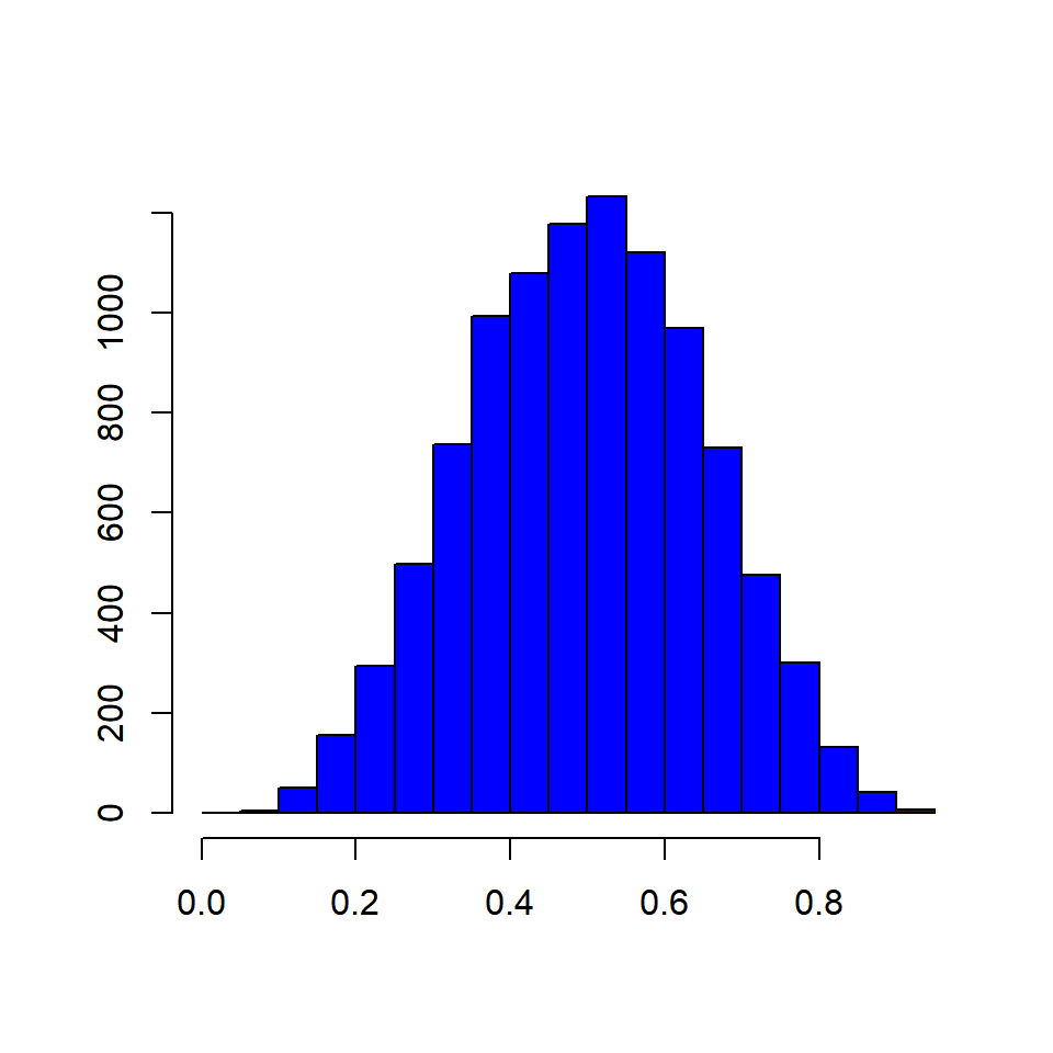
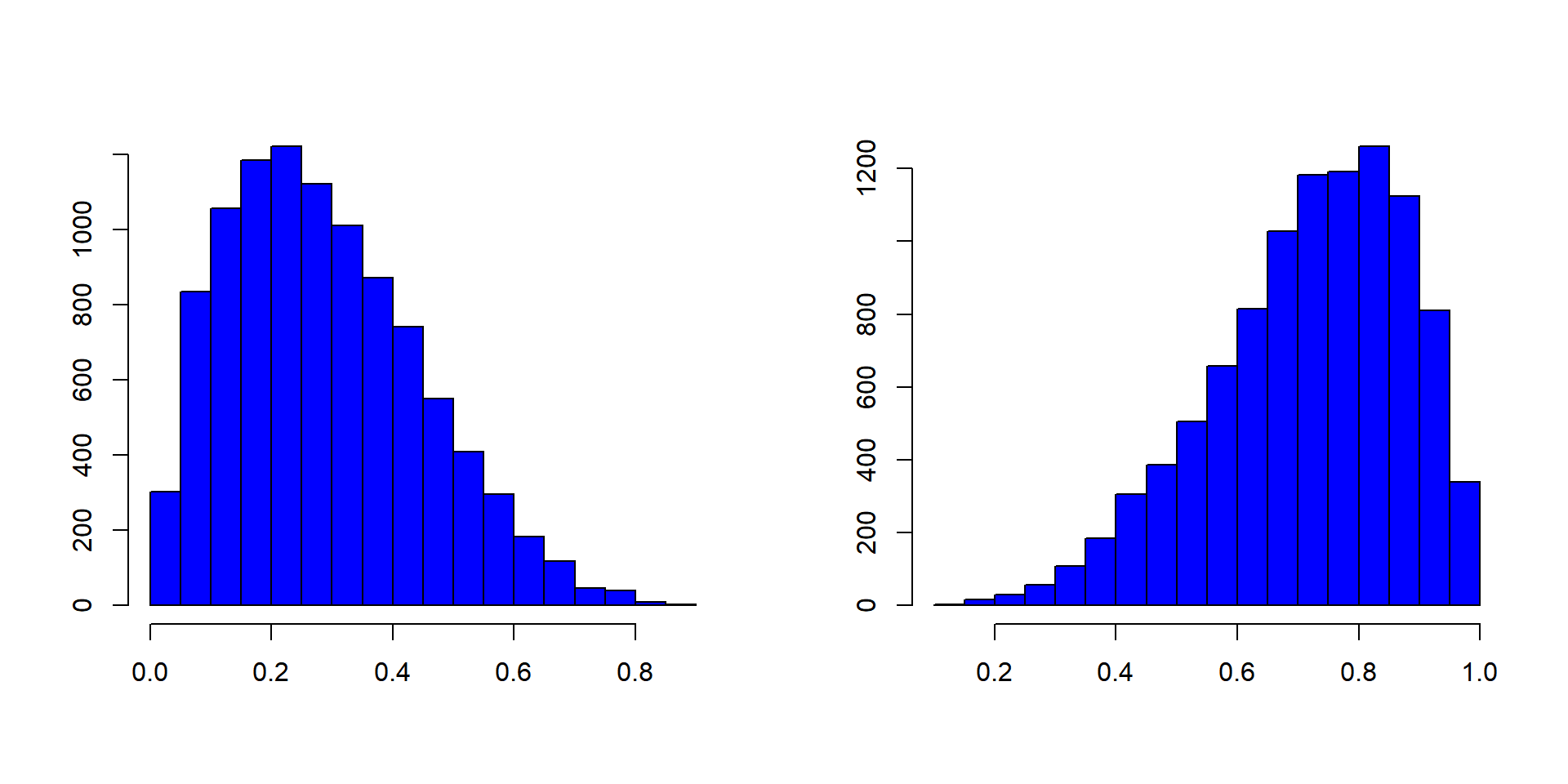
Before we learn how to create histograms, let us see how normal and skewed distributions look when represented by a histogram.
Normal Distribution
Skewed Distributions
Basics
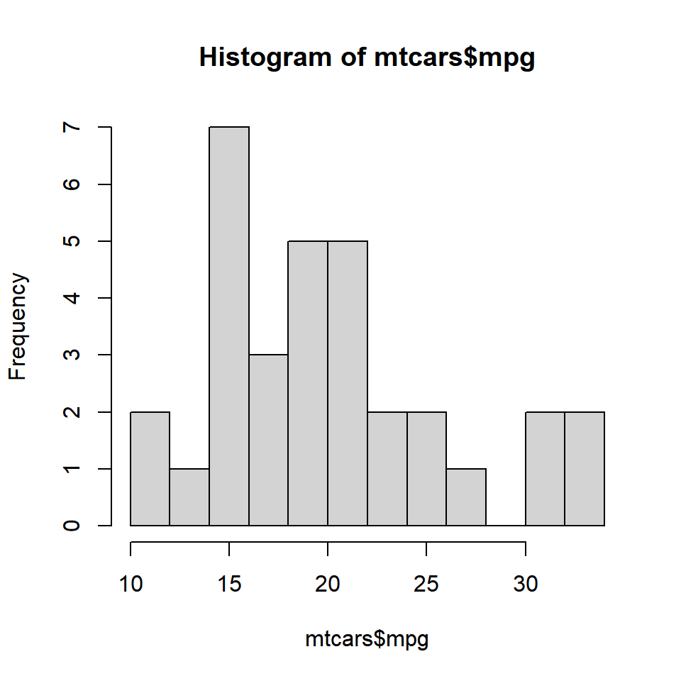
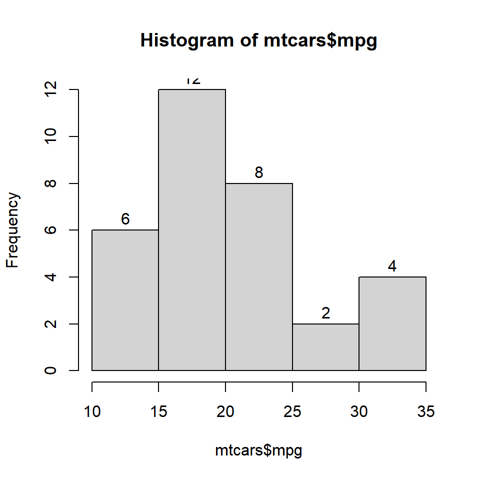
Histograms are created using the hist() function in R. The minimum input required to create a bare bones histogram is a continuous variable. Below is an example:
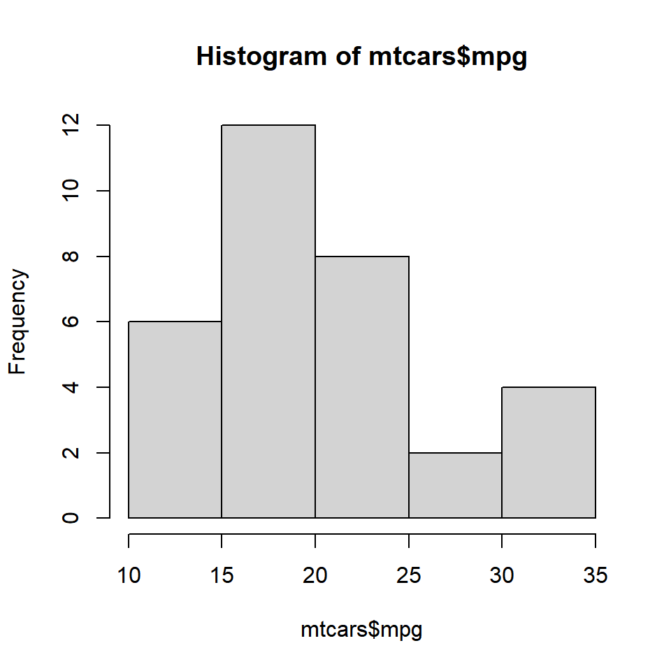
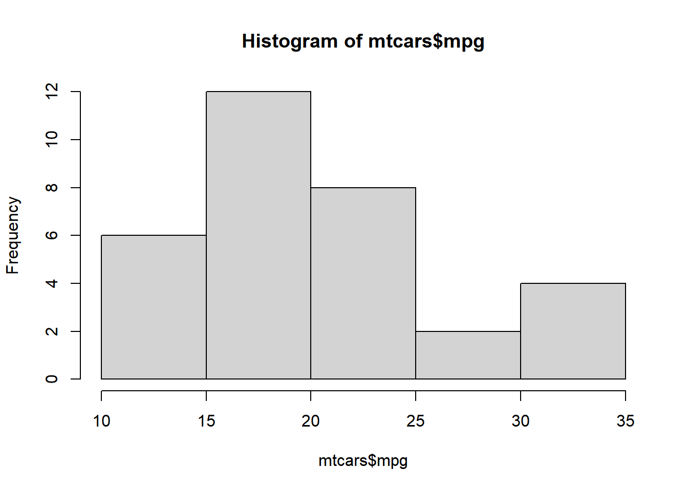
The hist() functions returns details of the histogram which can be accessed by assigning the histogram to a variable. Let us assign the above histogram to a variable h and use the \(</code> symbol to access the details stored in the variable.</p>
<pre class="r"><code># store the results of hist function
h <- hist(mtcars\)mpg)
# display number of breaks
h$breaks
## [1] 10 15 20 25 30 35

# frequency of the intervals
h$counts
## [1]  6 12  8  2  4

# frequency density
h$density
## [1] 0.0375 0.0750 0.0500 0.0125 0.0250

# mid points of the intervals
h$mids
## [1] 12.5 17.5 22.5 27.5 32.5

# varible name
h$xname
## [1] "mtcars$mpg"

# whether intervals are of equal size
h$equidist
## [1] TRUE