Code
install.packages("blorr")
blorr 0.3.2 is on CRAN. blorr provides tools for binary logistic regression in R: model fit statistics, variable selection, bivariate analysis, weight of evidence, and the validation charts used in credit scoring (gains table, ROC curve, KS chart and Lorenz curve), all built around glm() objects.
The last blorr post covered 0.2.0 in 2019. Since then there have been four CRAN releases (0.2.1, 0.2.2, 0.3.0 and 0.3.1), and this one changes numbers that may already be in reports:
If you report the Gini index, Cox–Snell or Nagelkerke R², or a likelihood ratio test from blorr, read the next three sections before you reuse those numbers. Everyone else can start at What is new since 2019.
You can install it from CRAN with:
install.packages("blorr")You can see a full list of changes in the release notes.
These fixes change results. In each case the new value agrees with the definition or with base R, so the new value is the one to report.
How we checked: Every number in this post was re-run against blorr 0.3.2 from CRAN; the release passed independent audits before submission.
Cox–Snell and Nagelkerke R² are functions of the fitted and intercept-only log-likelihoods and of the number of observations. If the data contain missing values, that number is the rows the model used, not the rows in the data frame.
bank_marketing records bank term-deposit marketing outcomes. It has no missing values, so we blank out 300 balances to mimic incomplete records:
bank_incomplete <- bank_marketing
set.seed(123)
bank_incomplete$balance[sample(nrow(bank_incomplete), 300)] <- NA
m_bank <- glm(y ~ balance + housing + loan, data = bank_incomplete, family = binomial)
c(rows_in_data = nrow(bank_incomplete), rows_fitted = nobs(m_bank))
rows_in_data rows_fitted
4521 4221 With \(n = 4221\) and the intercept-only model fitted on the same 4221 rows, the two R² values are:
n <- nobs(m_bank)
ll <- as.numeric(logLik(m_bank))
ll0 <- as.numeric(logLik(glm(y ~ 1, data = model.frame(m_bank), family = binomial)))
cox_snell <- 1 - exp((2 / n) * (ll0 - ll))
nagelkerke <- cox_snell / (1 - exp((2 / n) * ll0))
c(cox_snell = cox_snell, nagelkerke = nagelkerke)
cox_snell nagelkerke
0.02278596 0.04455730 blr_rsq_cox_snell() and blr_rsq_nagelkerke() return the same two values, and blr_model_fit_stats() prints them in the fit statistics table:
blr_model_fit_stats(m_bank) Model Fit Statistics
-----------------------------------------------------------------------------------
Log-Lik Intercept Only: -1511.502 Log-Lik Full Model: -1462.856
Deviance(4217): 2925.711 LR(3): 97.292
Prob > LR: 0.000
MCFadden's R2 0.032 McFadden's Adj R2: 0.030
ML (Cox-Snell) R2: 0.023 Cragg-Uhler(Nagelkerke) R2: 0.045
McKelvey & Zavoina's R2: 0.067 Efron's R2: 0.025
Count R2: 0.884 Adj Count R2: 0.000
BIC: 2959.102 AIC: 2933.711
-----------------------------------------------------------------------------------In 0.3.2 the intercept-only model keeps the fitted model’s response, offset and family/link, and n is nobs(model). Earlier versions used the number of rows in the data frame, so missing values pulled both R² towards zero.
What to do: re-run pseudo-R² for any model fitted with missing data; the new values are the ones that match the definitions.
The Gini index is usually reported beside the AUC in credit scoring, under the convention \(G = 2 \times \mathrm{AUC} - 1\). For the bank marketing model below, the ROC curve is:
m <- glm(y ~ duration + loan + housing + campaign, data = bank_marketing, family = binomial)
g <- blr_gains_table(m)blr_roc_curve(g)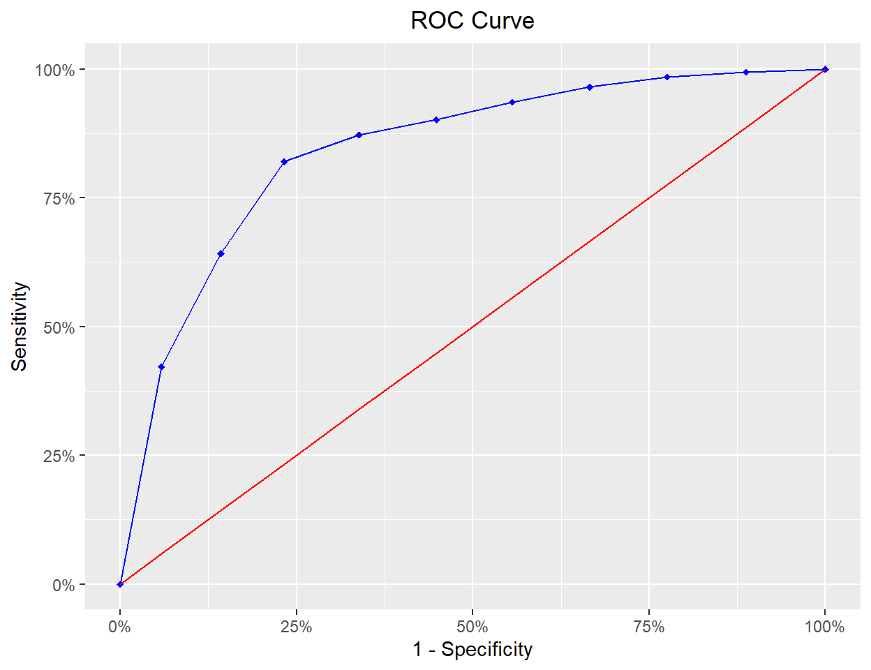
The area under that curve, computed from the ranks of the fitted probabilities, and the Gini index are:
p <- fitted(m)
event <- bank_marketing$y == "1"
r <- rank(p)
n1 <- sum(event)
n0 <- sum(!event)
auc <- (sum(r[event]) - n1 * (n1 + 1) / 2) / (n1 * n0)
c(auc = auc, gini_from_auc = 2 * auc - 1, gini = blr_gini_index(m))
auc gini_from_auc gini
0.8466918 0.6933835 0.6933835 The last two numbers are equal. In 0.3.2 blr_gini_index() computes the AUC from the Mann–Whitney rank statistic and returns \(2 \times \mathrm{AUC} - 1\), using only the rows the model was fitted on. Earlier versions returned the concentration index of the predicted probabilities, a different number for the same model, so a Gini reported before 0.3.2 cannot be compared with the AUC. The rank formula also avoids overflow on large models.
The gains table behind the curve now puts every observation in exactly one of ten deciles and counts events using the event level of the response:
c(observations = sum(g$gains_table$total), events = sum(g$gains_table$`1`))observations events
4521 517 What to do: recompute any Gini index and report it as \(2 \times \mathrm{AUC} - 1\) from now on.
A likelihood ratio test compares a full model with a reduced one. Its degrees of freedom are the difference in the number of estimated parameters, which is also the difference in residual degrees of freedom.
job has 12 levels, so adding it to a model with duration and loan adds 11 parameters:
m_red <- glm(y ~ duration + loan, data = bank_marketing, family = binomial)
m_full <- glm(y ~ duration + loan + job, data = bank_marketing, family = binomial)
c(resid_df_reduced = m_red$df.residual, resid_df_full = m_full$df.residual)
resid_df_reduced resid_df_full
4518 4507 The test uses those two residual degrees of freedom:
print(blr_test_lr(m_full, m_red)) Likelihood Ratio Test
------------------------------
Chi-Square DF Pr > ChiSq
------------------------------
86.2666 11 0.0000
------------------------------The same comparison in base R gives the same deviance, degrees of freedom and \(p\)-value:
anova(m_red, m_full, test = "Chisq")Analysis of Deviance Table
Model 1: y ~ duration + loan
Model 2: y ~ duration + loan + job
Resid. Df Resid. Dev Df Deviance Pr(>Chi)
1 4518 2644.9
2 4507 2558.7 11 86.267 8.951e-14 ***
---
Signif. codes: 0 '***' 0.001 '**' 0.01 '*' 0.05 '.' 0.1 ' ' 1In 0.3.2 the degrees of freedom come from df.residual of the two models, and the \(p\)-value from the chi-square distribution with those degrees of freedom. Earlier versions could report the wrong degrees of freedom, and therefore the wrong \(p\)-value, for nested models with factor predictors. The test also checks that the reduced model is nested in the full model by comparing the fitted design spaces instead of assuming it.
What to do: re-run likelihood ratio tests that involve factor predictors; a \(p\)-value from an earlier version may be based on the wrong degrees of freedom.
blorr’s tests and plots assume a binary response with a logit link. Version 0.3.2 checks the model before it calculates anything, instead of returning a number from a fit it cannot interpret:
m_q <- glm(y ~ duration, data = bank_marketing, family = quasibinomial)
blr_regress(m_q)
Error:
! blorr supports binary logistic regression only (binomial family, logit link). This model uses the 'quasibinomial' family and the 'logit' link.The same guard rejects prior weights other than 1, grouped binomial responses and fits stored without their model frame or response, and the selection functions reject these models before they refit anything.
The data behind the Lorenz curve and the decile capture-rate chart is exported as a plain data frame. blr_prep_lorenz_data() returns the cumulative event and non-event shares; blr_prep_dcrate_data() returns the decile counts and the decile mean:
head(blr_prep_lorenz_data(m), 4) cum_0s_per cum_1s_per
1 0.00000000 0.0000000
2 0.05844156 0.4216634
3 0.14285714 0.6421663
4 0.23276723 0.8201161head(blr_prep_dcrate_data(g), 4) decile total 1 decile_mean
1 1 452 218 0.48230088
2 2 452 114 0.25221239
3 3 452 92 0.20353982
4 4 452 27 0.05973451Both can go straight into ggplot2, plotly or any other plotting library, with the grouping and percentages already computed. The same applies to blr_prep_roc_data(), blr_prep_kschart_data() and blr_prep_kschart_stat().
blr_pairs() uses wide counters, so pair counts above the 32-bit integer limit no longer overflow, and its Somers’ D and Goodman–Kruskal gamma use the correct denominators.blr_eigen_cindex() sum to one, and condition indices stay finite for nearly collinear full-rank designs.blr_segment() and blr_segment_dist() is the share of events within each level.blr_woe_iv() accepts character and numeric predictors, drops unused factor levels, applies a 0.5 continuity correction to levels with no events or no non-events, and drops rows with missing values.These issues are known in 0.3.2. Most were found by an independent audit after the CRAN release. Each has a GitHub issue with a reproducible example, and each fix goes into blorr 0.3.3:
nlevels() of the response before fitting. Fixed on the development branch.blr_residual_diagnostics() uses the squared standardized Pearson residual (#146). Fixed on the development branch.blr_segment_twoway() are each cell’s share of all observations, not the event rate within the cell. For a within-cell rate, use tapply(y, list(a, b), mean) (#152).blr_segment() and blr_segment_dist() round proportions to two decimals before using them, so their percentages and plots can be off by up to half a percentage point (#153). For exact shares, use prop.table(table(x)) and tapply(y, x, mean).blr_woe_iv() adds up the rounded per-level values. For an accurate total, use a larger digits, for example digits = 4 (#155).Fixes for #152–#155 are on the development branch. blorr 0.3.3, with all of these fixes, is planned after 2027-01-13.
Thank you to everyone who contributed to blorr since the 2019 post by opening issues, reporting bugs and sending pull requests: @aravindhebbali, @DrMedfaresBrini, @Irazall, @LuiNov, @paleolimbot, and @romainfrancois.