ggplot2: Legend - Part 6

Title Alignment

The horizontal alignment of the title can be managed using the title.hjust argument. It can take any value between 0 and 1.

• 0 (left)
• 1 (right)

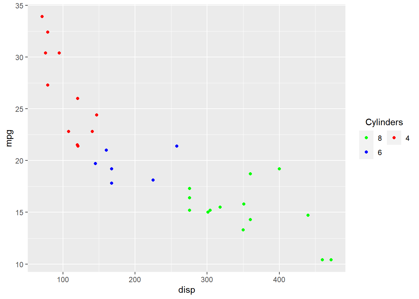
In the below example, we align the title to the center by assigning the value 0.5.

ggplot(mtcars) + geom_point(aes(disp, mpg, color = factor(cyl))) +
  scale_color_manual(values = c("red", "blue", "green"),
    guide = guide_legend(title = "Cylinders", title.hjust = 0.5))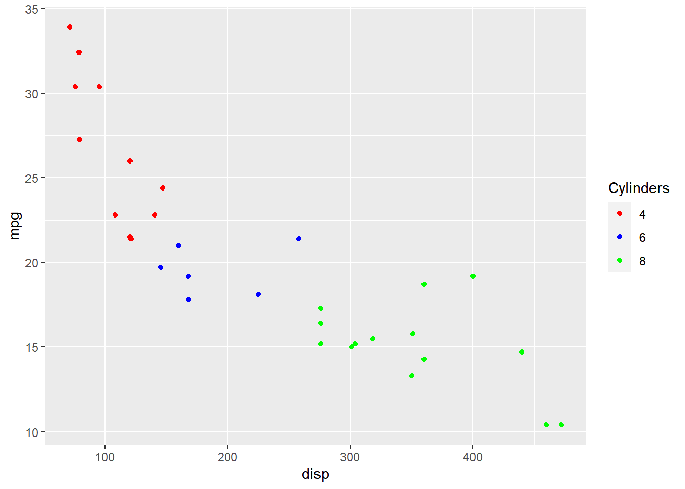

Title Alignment (Vertical)

To manage the vertical alignment of the title, use title.vjust.

ggplot(mtcars) + geom_point(aes(disp, mpg, color = hp)) +
  scale_color_continuous(guide = guide_colorbar(
    title = "Horsepower", title.position = "top", title.vjust = 1))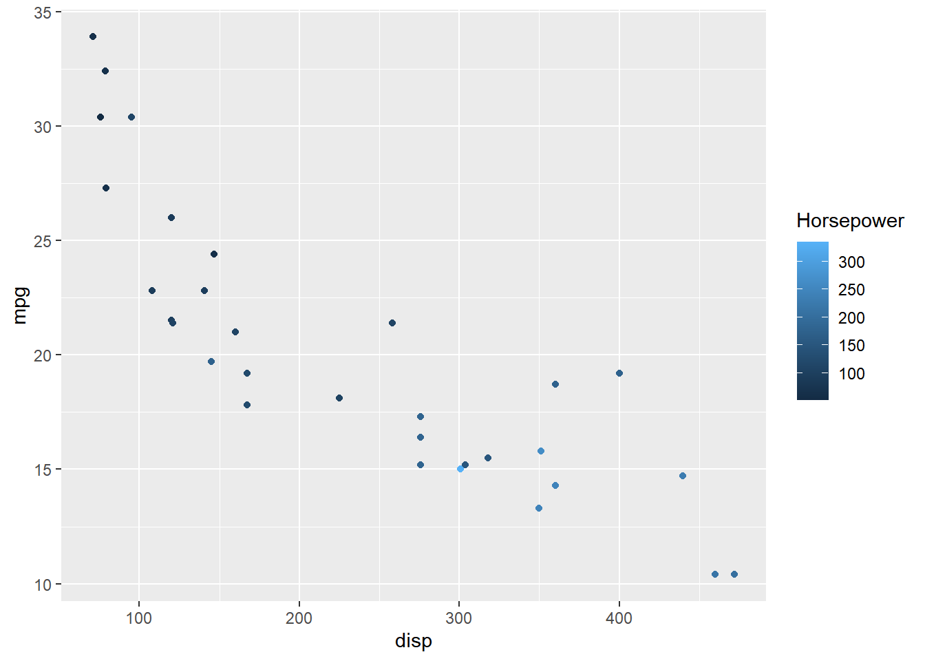

Title Position

The position of the title can be managed using title.posiiton argument. It can be positioned at:

• top
• bottom
• left
• right

ggplot(mtcars) + geom_point(aes(disp, mpg, color = factor(cyl))) +
  scale_color_manual(values = c("red", "blue", "green"),
    guide = guide_legend(title = "Cylinders", title.hjust = 0.5, 
      title.position = "top"))

Label Position

The position of the label can be managed using the label.position argument. It can be positioned at:

• top
• bottom
• left
• right

In the below example, we position the label at right.

ggplot(mtcars) + geom_point(aes(disp, mpg, color = factor(cyl))) +
  scale_color_manual(values = c("red", "blue", "green"),
    guide = guide_legend(label.position = "right"))

Label Alignment

The horizontal alignment of the label can be managed using the label.hjust argument. It can take any value between 0 and 1.

• 0 (left)
• 1 (right)

In the below example, we align the label to the center by assigning the value 0.5.

• alignment
  • 0 (left)
  • 1 (right)

ggplot(mtcars) + geom_point(aes(disp, mpg, color = factor(cyl))) +
  scale_color_manual(values = c("red", "blue", "green"),
    guide = guide_legend(label.hjust = 0.5))

ggplot(mtcars) +
  geom_point(aes(disp, mpg, color = hp)) +
  scale_color_continuous(guide = guide_colorbar(
    label.vjust = 0.8))

Direction

The direction of the label can be either horizontal or veritcal and it can be set using the direction argument.

ggplot(mtcars) + geom_point(aes(disp, mpg, color = factor(cyl))) +
  scale_color_manual(values = c("red", "blue", "green"),
    guide = guide_legend(direction = "horizontal"))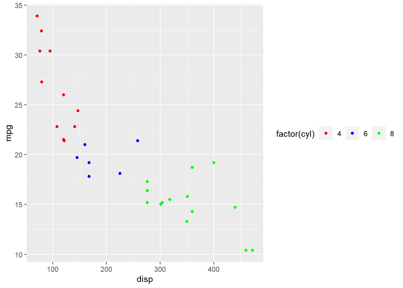

Rows

The label can be spread across multiple rows using the nrow argument. In the below example, the label is spread across 2 rows.

ggplot(mtcars) + geom_point(aes(disp, mpg, color = factor(cyl))) +
  scale_color_manual(values = c("red", "blue", "green"),
    guide = guide_legend(nrow = 2))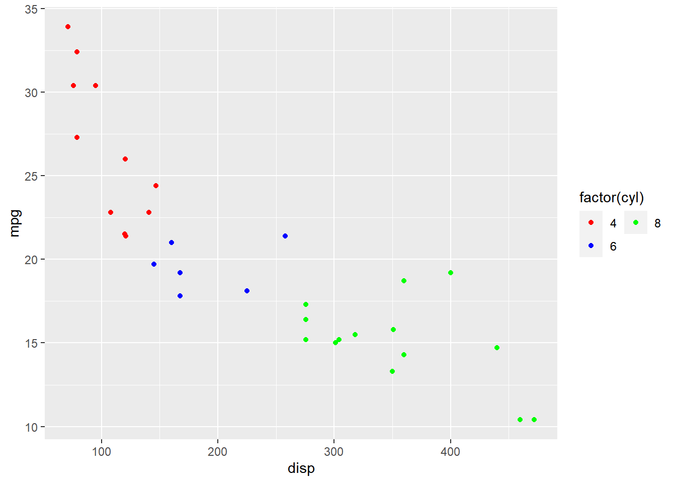

Reverse

The order of the labels can be reversed using the reverse argument. We need to supply logical values i.e. either TRUE or FALSE. If TRUE, the order will be reversed.

ggplot(mtcars) + geom_point(aes(disp, mpg, color = factor(cyl))) +
  scale_color_manual(values = c("red", "blue", "green"),
    guide = guide_legend(reverse = TRUE))

Putting it all together…

ggplot(mtcars) + geom_point(aes(disp, mpg, color = factor(cyl))) +
  scale_color_manual(values = c("red", "blue", "green"),
    guide = guide_legend(title = "Cylinders", title.hjust = 0.5, 
      title.position = "top", label.position = "right", 
      direction = "horizontal", label.hjust = 0.5, nrow = 2, reverse = TRUE)
  )

Legend Bar

So far we have looked at modifying components of the legend when it acts as a guide for color, fill or shape i.e. when the aesthetics have been mapped to a categorical variable. In this section, you will learn about guide_colorbar() which will allow us to modify the legend when the aesthetics are mapped to a continuous variable.

Plot

Let us start with a scatter plot examining the relationship between displacement and miles per gallon from the mtcars data set. We will map the color of the points to the hp variable.

ggplot(mtcars) +
  geom_point(aes(disp, mpg, color = hp))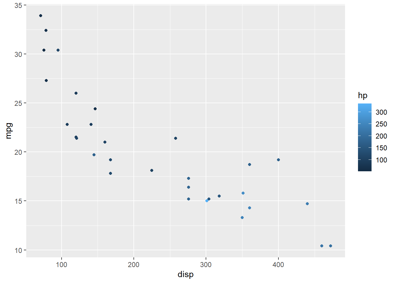

Width

The width of the bar can be modified using the barwidth argument. It is used inside the guide_colorbar() function which itself is supplied to the guide argument of scale_color_continuous().

ggplot(mtcars) +
  geom_point(aes(disp, mpg, color = hp)) +
  scale_color_continuous(guide = guide_colorbar(
    barwidth = 10))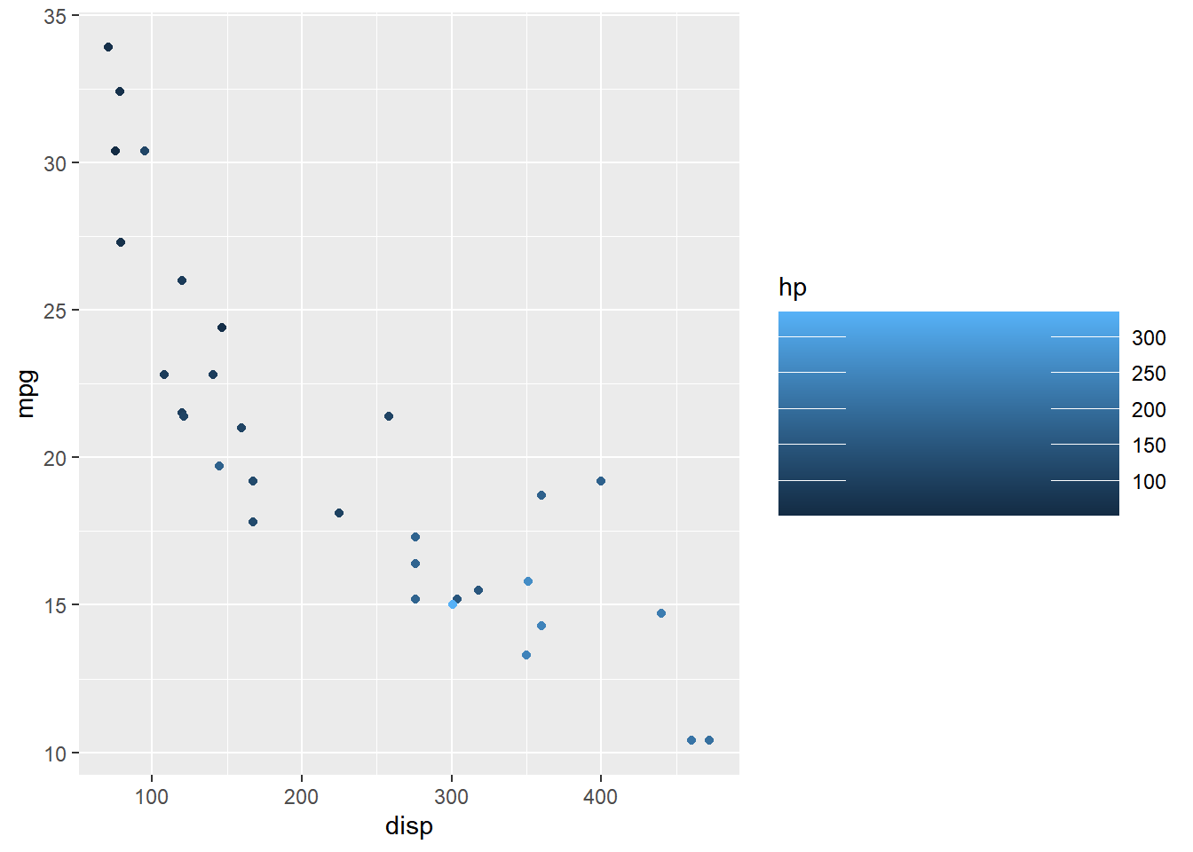

Height

Similarly, the height of the bar can be modified using the barheight argument.

ggplot(mtcars) +
  geom_point(aes(disp, mpg, color = hp)) +
  scale_color_continuous(guide = guide_colorbar(
    barheight = 3))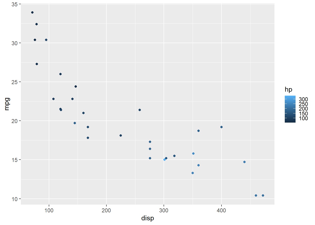

Bins

The nbin argument allows us to specify the number of bins in the bar.

ggplot(mtcars) +
  geom_point(aes(disp, mpg, color = hp)) +
  scale_color_continuous(guide = guide_colorbar(
    nbin = 4))

Ticks

The ticks of the bar can be removed using the ticks argument and setting it to FALSE.

ggplot(mtcars) +
  geom_point(aes(disp, mpg, color = hp)) +
  scale_color_continuous(guide = guide_colorbar(
    ticks = FALSE))

Upper/Lower Limits

The upper and lower limits of the bars can be drawn or undrawn using the draw.ulim and draw.llim arguments. They both accept logical values.

ggplot(mtcars) +
  geom_point(aes(disp, mpg, color = hp)) +
  scale_color_continuous(guide = guide_colorbar(
    draw.ulim = TRUE, draw.llim = FALSE))

Guides: Color, Shape & Size

The guides() function can be used to create multiple legends to act as a guide for color, shape, size etc. as shown below. First, we map color, shape and size to different variables. Next, in the guides() function, we supply values to each of the above aesthetics to indicate the type of legend.

ggplot(mtcars) +
  geom_point(aes(disp, mpg, color = hp, 
    size = qsec, shape = factor(gear))) + 
  guides(color = "colorbar", shape = "legend", size = "legend")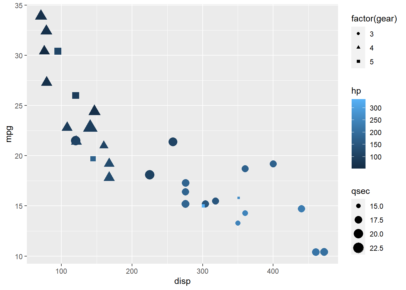

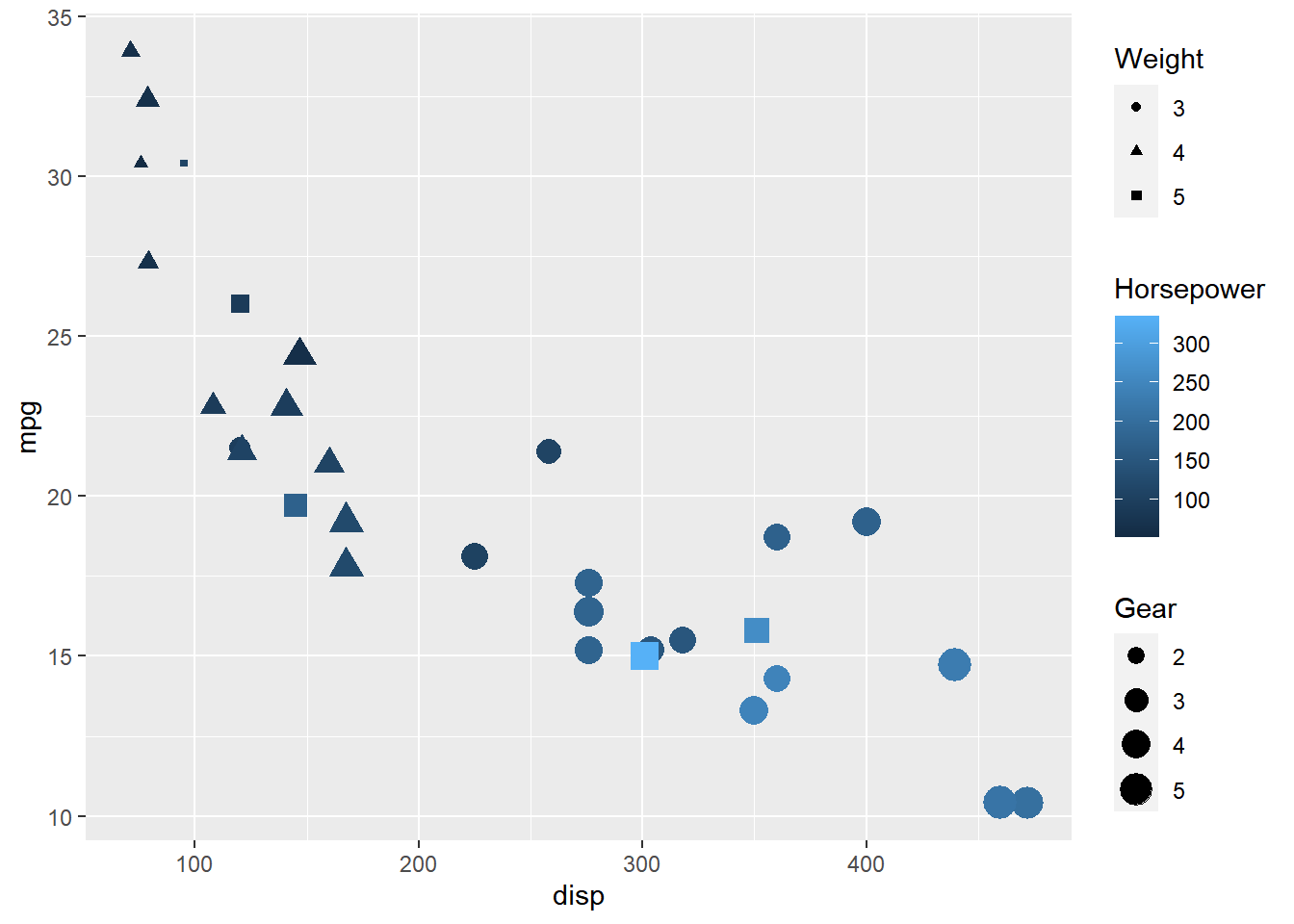
Guides: Title

To modify the components of the different legends, we must use the guide_* family of functions. In the below example, we use guide_colorbar() for the legend acting as guide for color mapped to a continuous variable and guide_legend() for the legends acting as guide for shape/size mapped to categorical variables.

ggplot(mtcars) +
  geom_point(aes(disp, mpg, color = hp, size = wt, shape = factor(gear))) + 
  guides(color = guide_colorbar(title = "Horsepower"),
    shape = guide_legend(title = "Weight"), size = guide_legend(title = "Gear")
  )

Summary

In this post, we will learn to modify legend

• title
• label
• and bar

Up Next..

In the next post, we will learn faceting.