Introduction
This is the second post in the series Elegant Data Visualization with
ggplot2. In the previous post, we understood the concept of grammar of
graphics and even built a bar plot step by step while exploring the different
components of a plot/chart. In this post, we will learn to quickly build a set
of plots that are routinely used to explore data using qplot(). It can be
used to quickly create plots but also has certain limitations. Nevertheless, if
you want to quickly explore data using a single function, qplot() is your friend.
Libraries, Code & Data
We will use the following libraries in this post:
All the data sets used in this post can be found here and code can be downloaded from here.
Scatter Plot
Scatter plots are used to examine the relationship between two continuous variables. The relationship can be examined across the levels of a categorical variable as well. Let us begin by creating scatter plots. The first two inputs are the variables/columns representing the X and Y axis. The next input is the name of the data set.
qplot(disp, mpg, data = mtcars)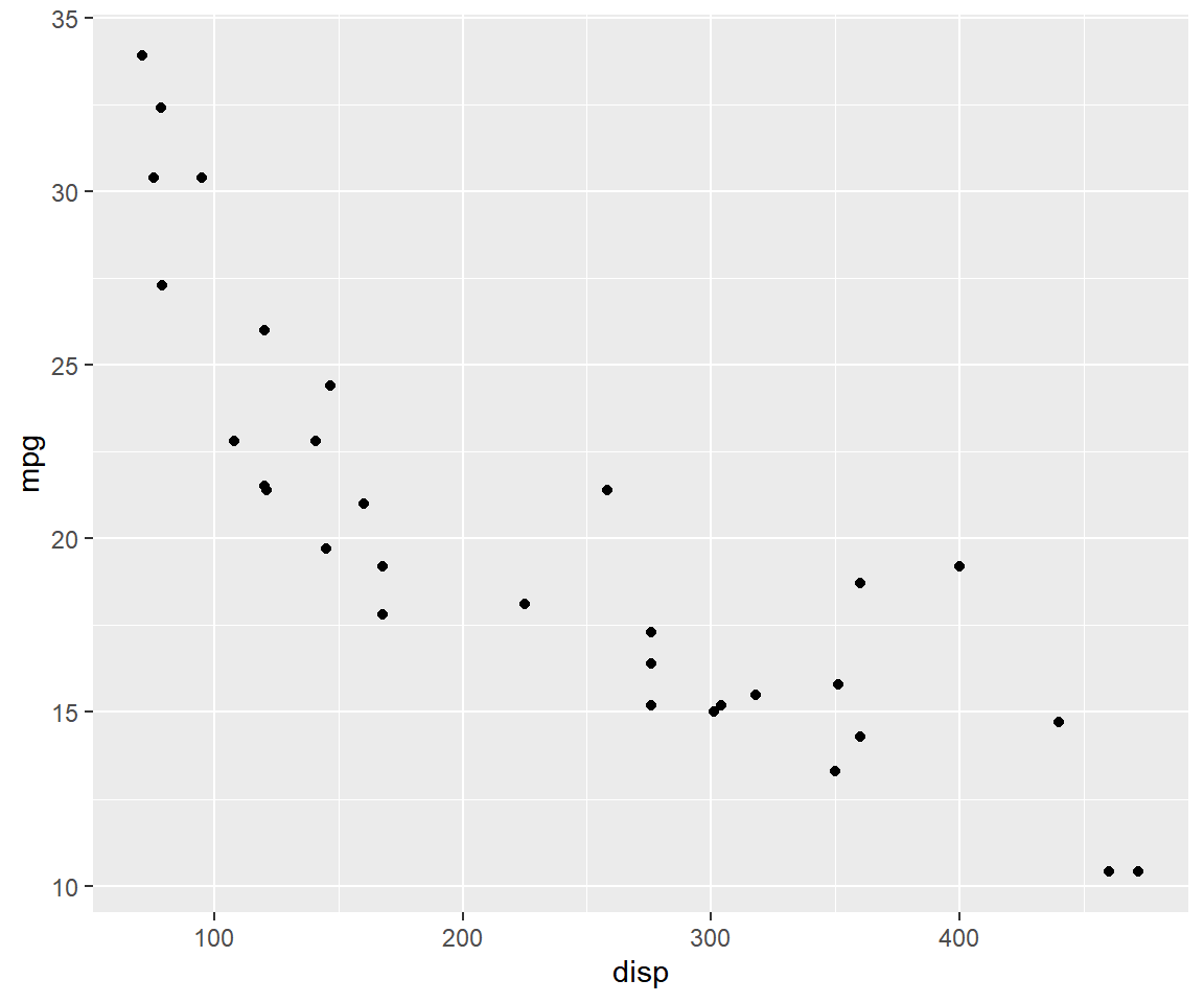
If you want the relationship between the two variables to be represented by
both points and line, use the geom argument and supply it the values using a
character vector.
qplot(disp, mpg, data = mtcars, geom = c('point', 'line'))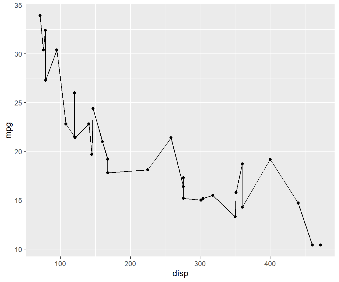
The color of the points can be mapped to a categorical variable, in our case
cyl, using the color argument. Ensure that the variable is categorical using
factor().
qplot(disp, mpg, data = mtcars, color = factor(cyl))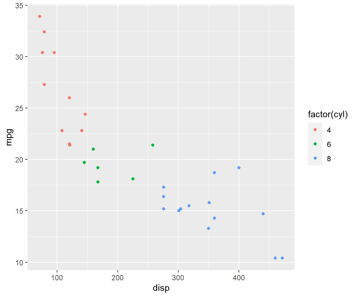
The shape and size of the points can also be mapped to variables using the
shape and size argument as shown in the below examples.
qplot(disp, mpg, data = mtcars, shape = factor(cyl))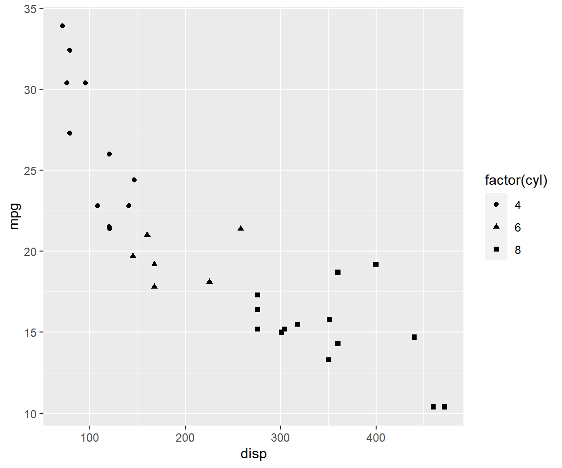
Ensure that size is mapped to a continuous variable.
qplot(disp, mpg, data = mtcars, size = qsec)
Bar Plot
A bar plot represents data in rectangular bars. The length of the bars are proportional to the values they represent. Bar plots can be either horizontal or vertical. The X axis of the plot represents the levels or the categories and the Y axis represents the frequency/count of the variable.
To create a bar plot, the first input must be a categorical variable. You can
convert a variable to type factor (R equivalent of categorical) using the
factor() function. The next input is the name of the data set and the final
input is the geom which is supplied the value 'bar'.
qplot(factor(cyl), data = mtcars, geom = c('bar'))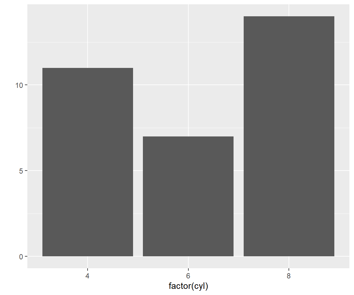 You can create a stacked bar plot using the
 fill argument and mapping it to
another categorical variable.
qplot(factor(cyl), data = mtcars, geom = c('bar'), fill = factor(am))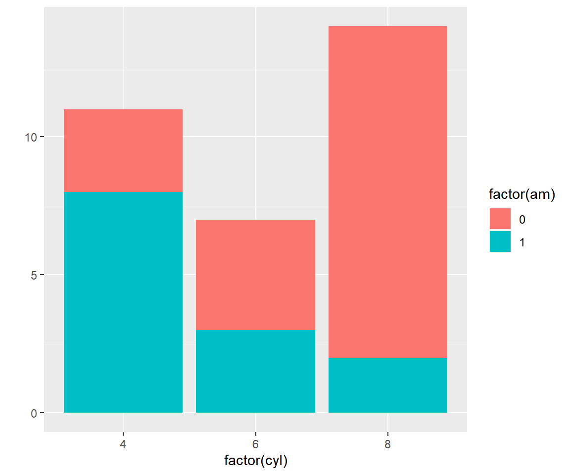
Box Plot
The box plot is a standardized way of displaying the distribution of data based on the five number summary: minimum, first quartile, median, third quartile, and maximum. Box plots are useful for detecting outliers and for comparing distributions. It shows the shape, central tendancy and variability of the data.
Box plots can be created by supplying the value 'boxplot' to the geom
argument. The firstinput must be a categorical variable and the second must be
a continuous variable.
qplot(factor(cyl), mpg, data = mtcars, geom = c('boxplot'))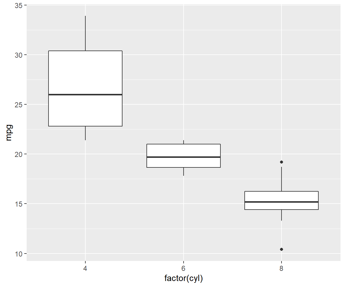
Unlike plot(), we cannot create box plots using a single variable. If you are
not comparing the distribution of a variable across the levels of a categorical
variable, you must supply the value 1 as the first input as show below.
qplot(factor(1), mpg, data = mtcars, geom = c('boxplot'))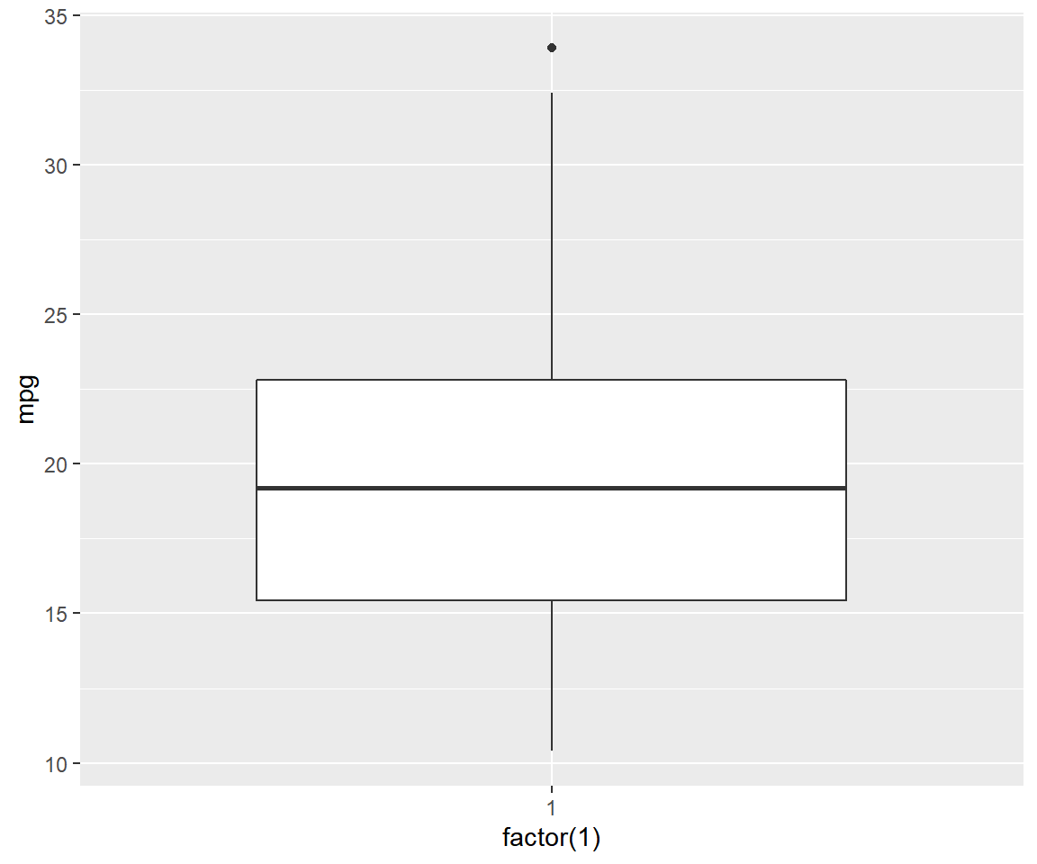
Line Chart
Line charts are used to examing trends across time. To create a line chart,
supply the value 'line' to the geom argument. The first two inputs should
be names of the columns/variables representing the X and Y axis, and the third
input must be the name of the data set.
qplot(x = date, y = unemploy, data = economics, geom = c('line'))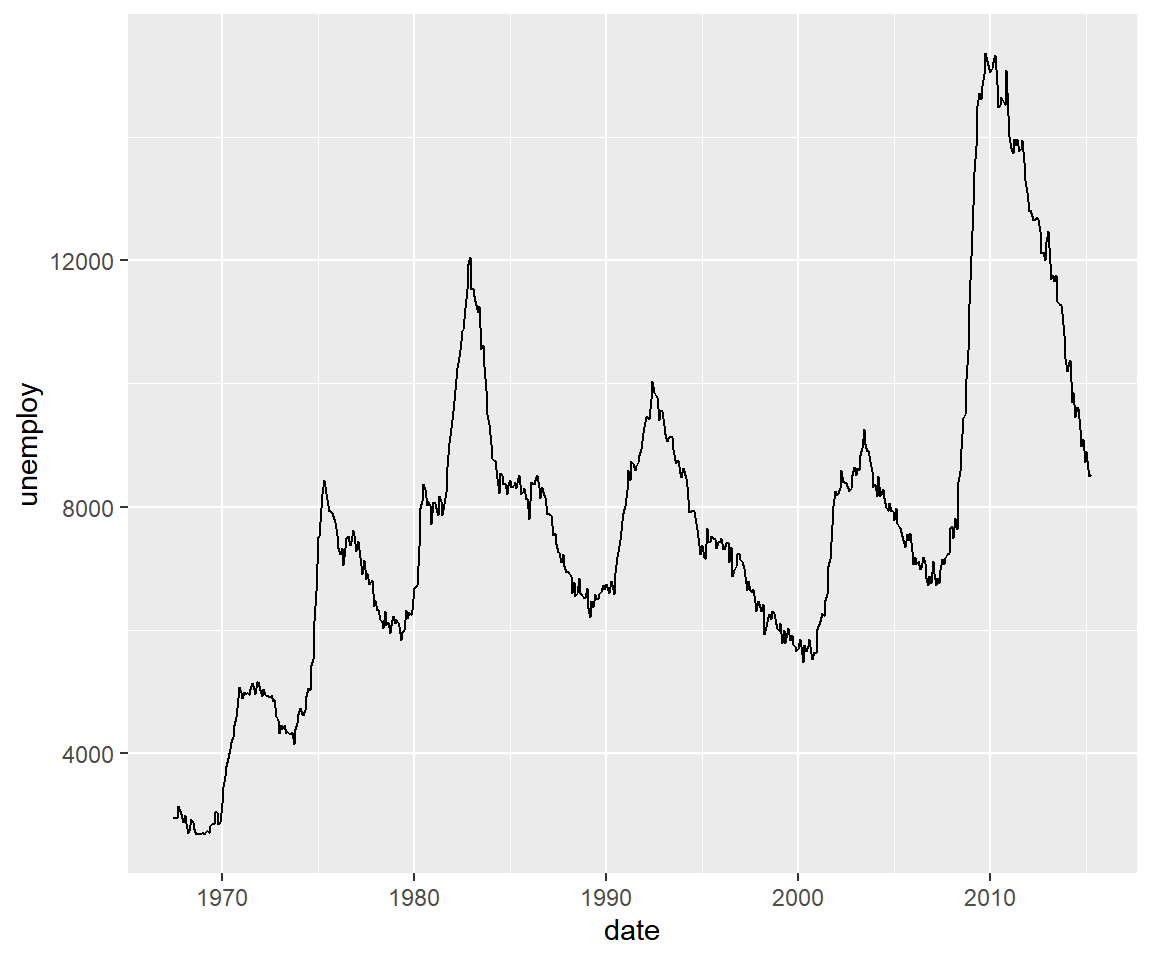
The appearance of the line can be modified using the color argument as shown below.
qplot(x = date, y = unemploy, data = economics, geom = c('line'),
      color = 'red')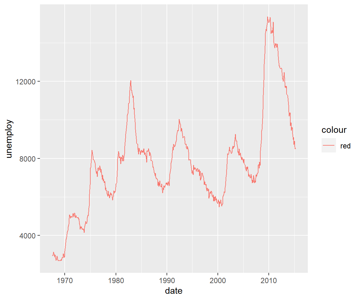
Histogram
A histogram is a plot that can be used to examine the shape and spread of
continuous data. It looks very similar to a bar graph and can be used to detect
outliers and skewness in data. A histogram is created using the bins argument
as shown below. The first input is the name of the continuous variable and the
second is the name of the data set.
qplot(mpg, data = mtcars, bins = 5)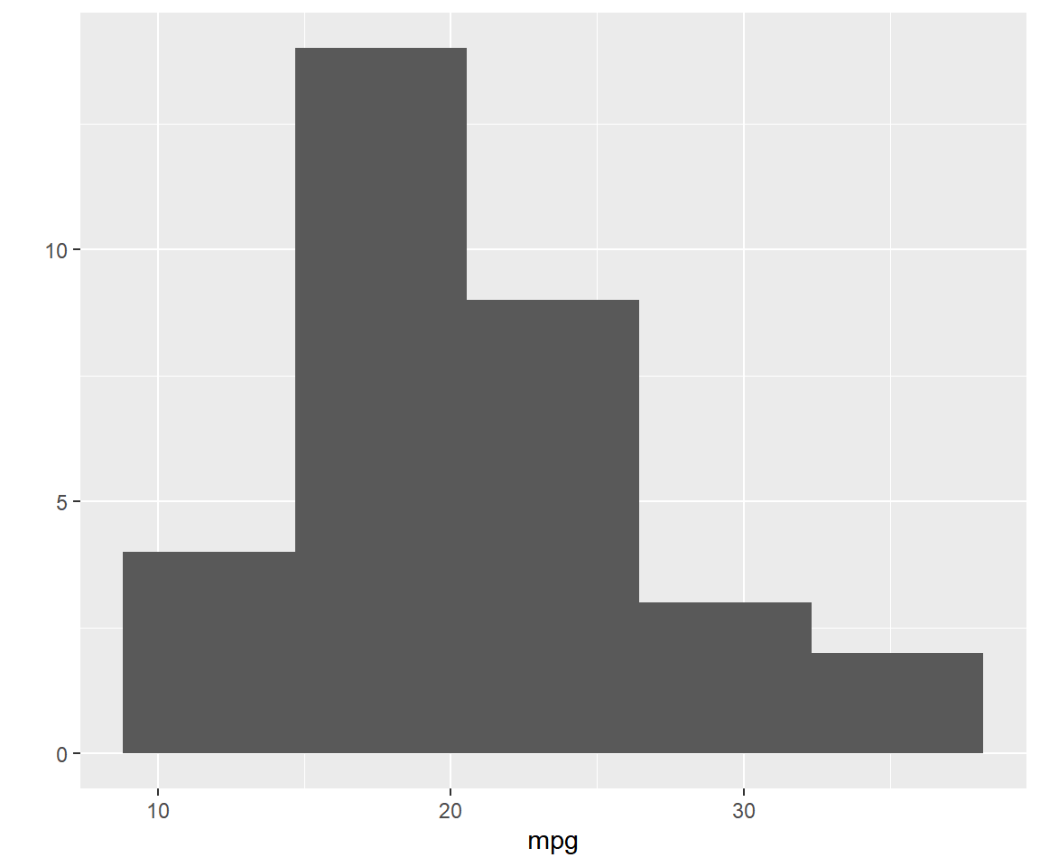
Summary
In this post, we learnt to quickly create plots using the qplot() function. While useful, it has limitations and can be used only to quickly visualize data.
Up Next..
In the next post, we will create the same set of plots but using geoms.