
Introduction
In a previous post, we had introduced our R package rfm but did not go into the conceptual details of RFM analysis. In this post, we will explore RFM in much more depth and work through a case study as well. RFM (Recency, Frequency & Monetary) analysis is a behavior based technique used to segment customers by examining their transaction history such as:
- how recently a customer has purchased?
- how often do they purchase?
- how much the customer spends?
It is based on the marketing axiom that 80% of your business comes from 20% of your customers. RFM helps to identify customers who are more likely to respond to promotions by segmenting them into various categories.
Resources
Below are the links to all resources related to this post:
You can try our free online course Customer Segmentation using RFM Analysis if you like to learn through self paced online courses.
Case Study
We will work through a case study to better understand the underlying concepts of RFM analysis. To pique your curiosity, we will start with the results or the final outcome of the case study as shown below:

The table has the following details:
- name or id of the customer
- number of days since the last transaction of the customer
- number of transactions of the customer
- total value of the all the transactions of the customer
- RFM score
- customer segment
The rest of this post will focus on generating a similar result for our case study and along the way we will learn to:
- structure data for RFM analysis
- generate RFM score
- and segment customers using RFM score
Applications

Let us talk about applications. Though largely identified with retail or ecommerce, RFM analysis can be applied in a lot of other domains or industry as well. In social media and apps, RFM can be used to segment users as well. The only difference is instead of using monetary value as the third metric, we will use the amount of time spent (or some other metric based on it) on the site/app. The more time we spend on the platform and consume the content, the more ads can be displayed by the platform. So in those cases, the amount of time we spend will be the third metric.
RFM Workflow
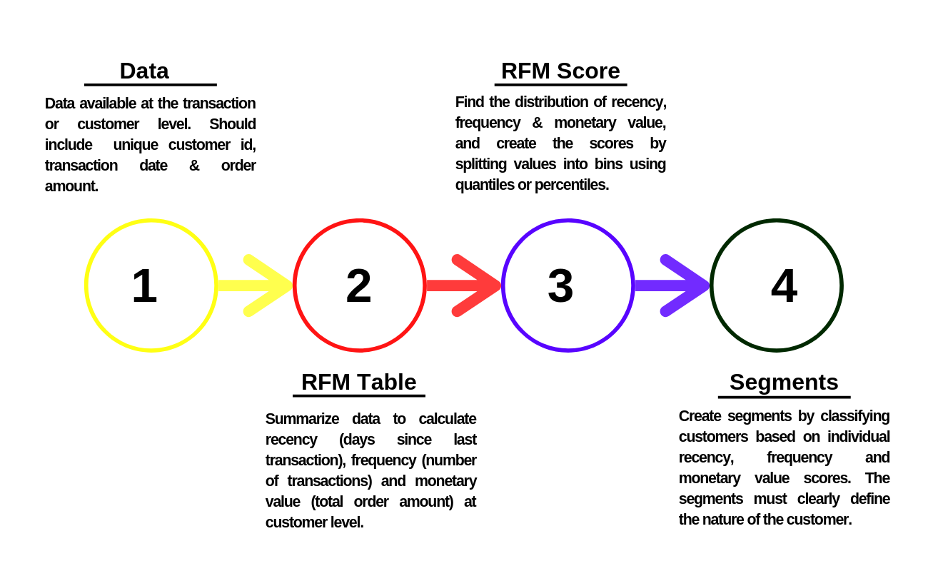
The typical workflow for RFM analysis is shown above. It can be broadly divided into the following:
In the first step of the workflow, we collect transaction data. This should include a unique customer id, transaction date and transaction amount. In case of ecommerce, we need to decide how to treat visits that did not result in a transaction. If data is aggregated and made available at the customer level, it must include a unique customer id, last transaction date and total revenue from the customer. The last transaction date may be replaced by days since last visit as well. The details available in data supplied depends on the data pipeline and the
rfmpackage can handle any of the above 3 scenarios.In the second step, we generate RFM table from the raw data available. The RFM table aggregates data at the customer level. It includes the unique customer id, days since last transaction/visit, frequency of transactions/visits and the total revenue from all the transactions of the customer.
In the third step, we generate scores for recency, frequency and monetary value, and use them to create the RFM score for each customer.
In the final step, we use the recency, frequency and monetary scores to define customer segments and design customised campaigns, promotions, offers & discounts to retain and reactivate customers.
RFM Table
Let us assume we have completed the first step in RFM analysis by collecting transaction data. Now, we have to generate the RFM table from the transaction data. In the transaction data, each row represents a transaction and we may get the transaction details in any of the following ways:
- according to transaction date
- sorted by customer id
- or in a random order
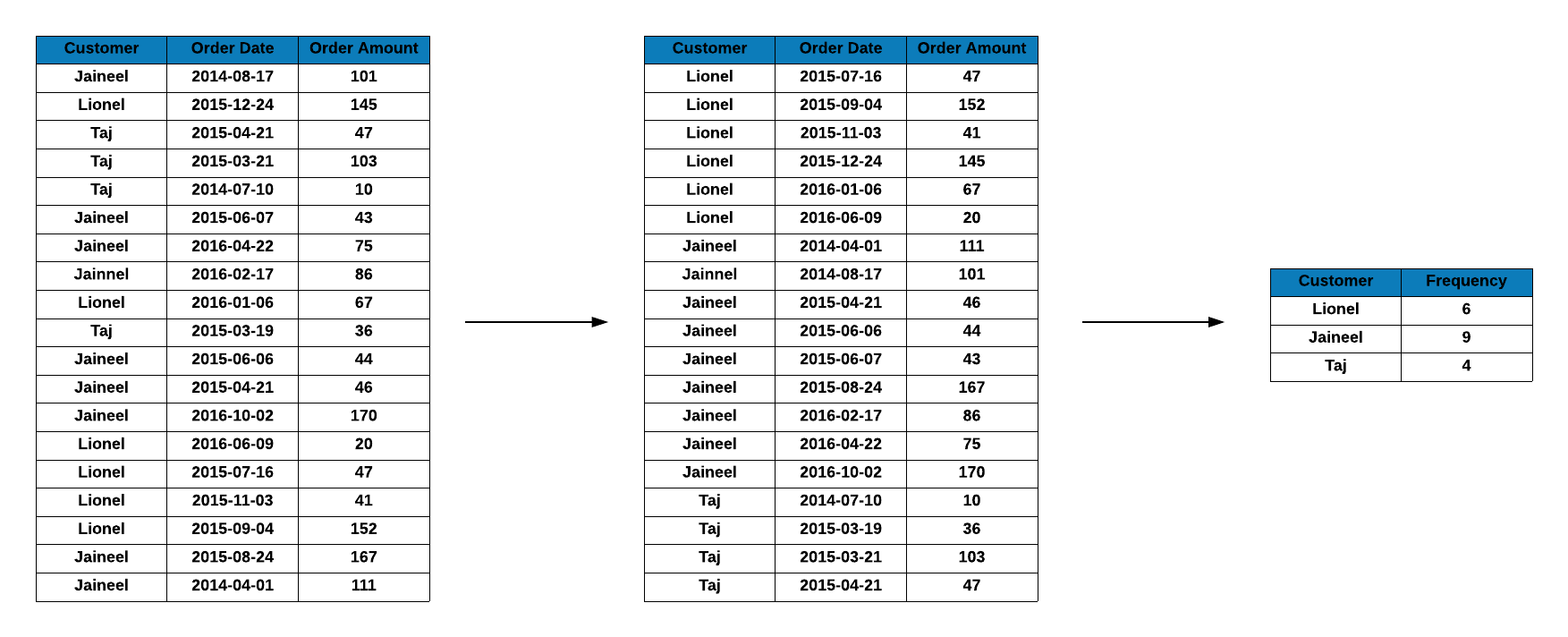
The first two cases are more likely but if we get the transaction data in a random order, the first order of business is to sort them by customer id. In the below example, we have transaction details for 3 customers Lionel, Jaineel and Taj but they are not sorted by transaction date or customer id. Since we want to create the RFM table from this data, we sort it by customer id.
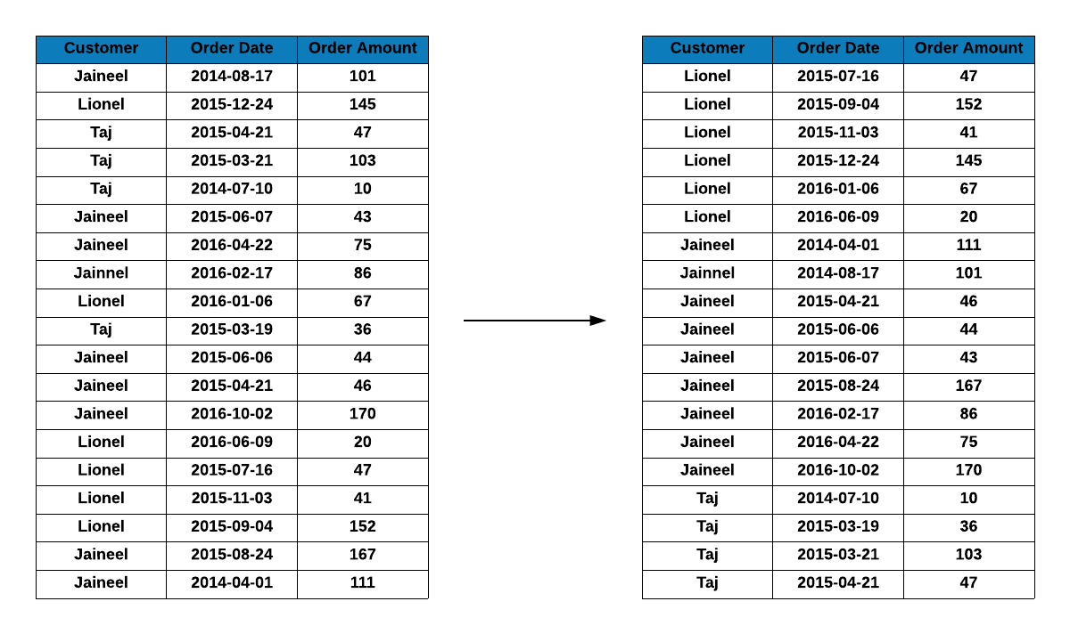
From the sorted data, we aggregate the transaction details at the customer level as shown below.
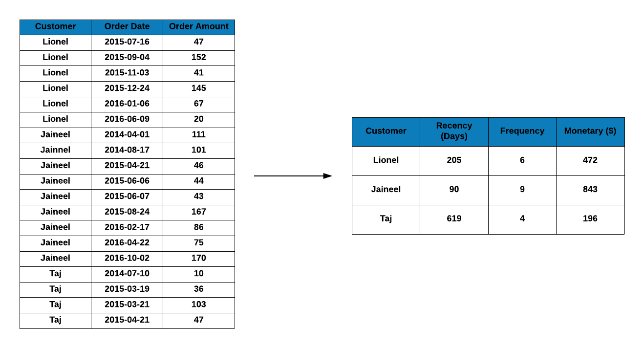
From the above step, we have created the RFM table which contains recency (days since last visit), frequency (frequency of visits) and monetary (total revenue from the customer) data for each customer.

Metrics
Time to talk about the key metrics Recency, Frequency and Monetary in more detail. In this section, we will understand how they are calculated, and in the next section, we will learn how they are used for generating the RFM score.
Recency
Let us begin with recency. Earlier, we defined it as the number of days since the last transaction of the customer. How do we calculate this metric? Apart from the date of the last transaction of the customer, what other information do we need? In all the discussions till now, we have missed out on a key point i.e. the time frame of the analysis.
The most crucial step in RFM analysis is to select a time frame from which we use the transaction data. How do we decide on this time frame? It depends on the domain to which we are applying this analysis. Customers visit a grocery store more often than they visit a consumer durables store. Similarly, people consume content from news & blogs more frequently while they may visit an e-commerce website only when they have to purchase something. Keeping in mind the domain to which the analysis is being applied, select an appropriate time frame. To calculate recency, compute the difference between the last transaction date and the analysis date i.e. the last date of the selected time frame.
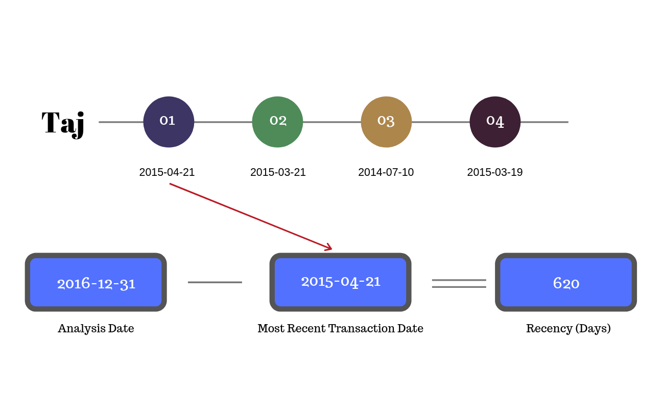
In the above example, the analysis date is 2016-12-31. To compute recency,
we first extract all the transaction date of customer Taj and then select the
last transaction date, 2015-04-21, and subtract if from the analysis
date to get the number of days since the last transaction date, 620.
Frequency
Frequency is the count of transactions. In the online/digital world, we need to decide whether we will consider all the visits to a website or app as the frequency or only those which resulted in a transaction/conversion. In the below example, we count the transactions for each customer and use it as frequency. Lionel has 6 transactions, Jaineel has 9 transactions and Taj has 4 transactions.
Monetary Value
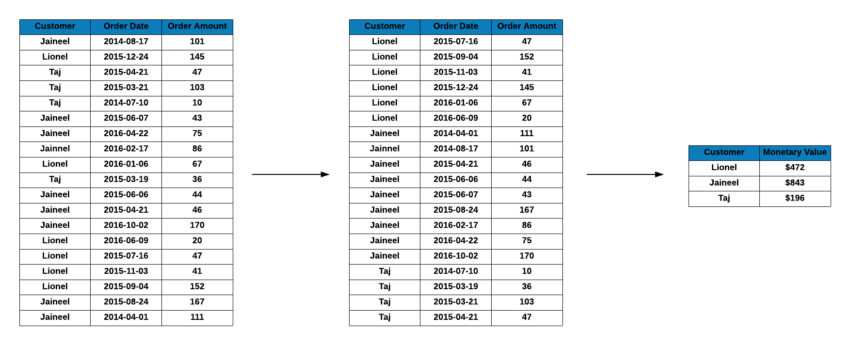
Monetary value is the total revenue from each customer in the selected time
frame. It is computed by summing up the transaction amount. In our case study,
Jaineel has spent the highest amount of $843, followed by Lionel who has
spent $472 and Taj has spent the lowest, $196. As you can observe, we have
arrived at these figures by summing the values in the third column of the
second table, Order Amount.
If we are applying this analysis to the digital world, we may think of using a metric such as time spent on the website/app instead of transaction/order amount.
RFM Score
As shown in the workflow, the third step in RFM analysis is to generate the individual score for each metric and then use them to generate the RFM score. In this section, we will explain in detail how the scores are computed for recency, frequency and monetary. This section is slightly complex (we received a lot of mails from readers after we published the previous post) and we have tried our best to break down the complexity as much as possible. Still, if you have any questions feel free to write to us at support@rsquaredacademy.com.
We follow the below steps to create the score:
- use quantiles to generate cut off points
- create intervals based on the cut off points
- use the intervals to assign score
Monetary Score
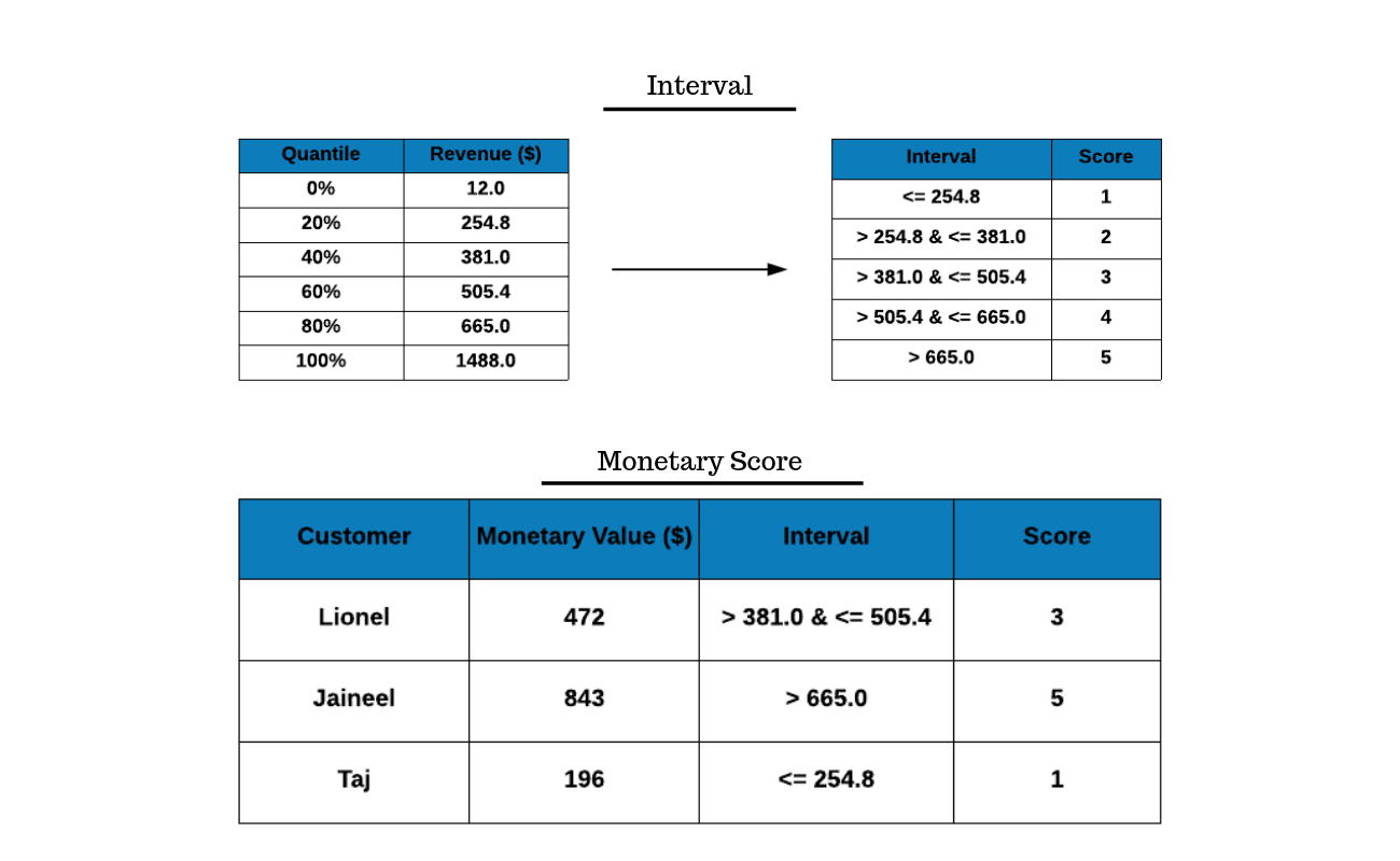
Let us generate the monetary score in our case study. The first step is to
compute the quantiles using the quantile() function. We use the revenue
column from the RFM table to compute the quantiles. If you look at the example,
it gives us the cut off below which a certain percentage of customers are
present.
- the bottom 20% of customers spend below
$254.8. - the next 20% of customers spend between
$254.8and$381.0. - the top 20% of customers spend above
$665.0.
Using these cut off points we have created intervals which can then be converted
to if else statements. The intervals are then used to assign scores. For
example, Lionel falls in the interval > 381.0 & <= 505.4 and hence is assigned
the score 3. Similarly, Jaineel and Taj are assigned the scores 5 and 1.
How do we interpret the scores? The score is more like a rank. A customer with
a score of 3 is ranked higher than a customer with score of 1 as his transaction
amount is higher. In the rfm package, we use the above method to assign the
scores.
Some users reverse the order of the score i.e. top 20% customers by transaction amountare assigned the score 1 and the bottom 20% are assigned the score 5.
Frequency Score
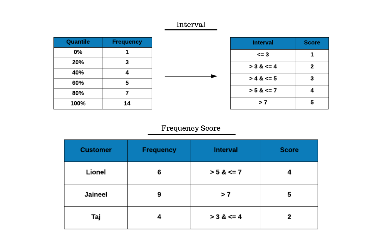
The frequency score is computed in the same way as the monetary score. Instead of using the revenue column from the RFM table, we use the frequency column. Using quantiles, we arrive at the cut off points below which a certain percentage of customer are present. If you observe the example, the first table shows the quantiles and the associated cut off points.
- the bottom 20% of customers visit/transact less than 3 times.
- the next 20% of customers visit/transact around 4 times.
- the top 20% of customers visit/transact more than 7 times.
The cut off points are then used to create the intervals and assign the scores as shown in the second table. We assign a higher score to those who visit more frequently and a lower score to those who visit less frequently.
In our case study, Jaineel has visited 9 times and hence assigned the score 5 where as Taj has visited only 4 times and hence the score 2.
Recency Score
The recency score follows the same methodology but uses a slightly different concept while assigning the score. If you look at the metrics, the higher the values of frequency and monetary, the better as we want customers to transact frequently and spend higher amount but it is not the case with recency. Since recency represents the number of days since the last transaction, the lower its value the better i.e. customers who visited in the recent past are more likely to visit again whereas customers who visited long back may be as good as lost. Hence in the case of recency, higher score is assigned to those with lower recency value and vice versa.
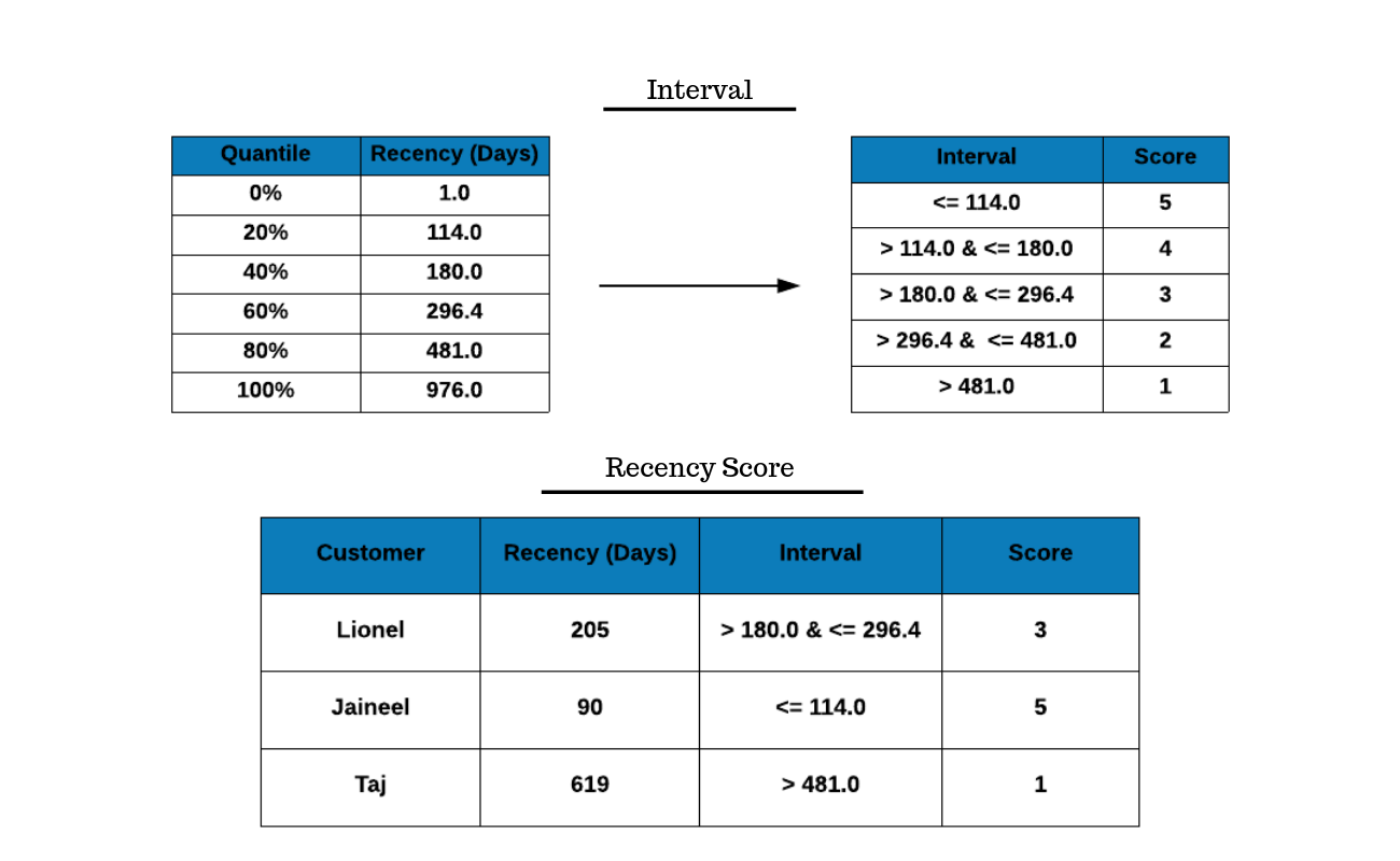
In the above example, we have used quantiles to compute the cut off point for recency. The first table shows the quantiles and the associated cut off points:
- the bottom 20% of customers visited more than
481days back. - the next 20% of customers visited between
296.4and481days back. - the top 20% of customers visited less than 114 days back.
The above statements will become clear if you study the second table which includes the interval and the score. We have assigned a higher score to those who visited in the recent past (< 114 days) compared to those who visited way back (> 481 days). In our case study, Jaineel visited in the past 3 months and hence the score of 5 where as Taj visited almost 20 months back and has been assigned the score 1.
RFM Score
Now that we have calculated the individual scores, let us compute the RFM score using the below formula:
RFM Score = Recency Score * 100 + Frequency Score * 10 + Monetary Score
The below table shows the individal scores of recency, frequency and monetary as well as the RFM score. All of them are computed from the RFM table which in itself is based on the transaction data.

Segments
Great! We have finally computed the RFM score. Now what? How do we define the segments using this score? In this section, we will learn how to define customer segments using the RFM score. The below table is an example of how segments are defined. It has the following details:
- the name of the segment
- the definition of the segment
- the intervals for the recency, frequency & monetary scores
We should be careful while creating the intervals for the scores in the segments table. Look at this Wkipedia article to understand how intervals work.
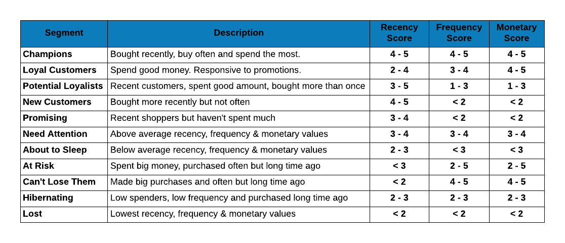
Let us apply the above rules to our case study.

Defining segments is another crucial step in RFM analysis. We need to ensure
that there is no duplication or large number of customers get classified into
Others segment. In the case study, we will show you some of the mistakes
that can happen while defining the segments.
Case Study
It is time to work through the case study. Let us first load all the libraries we will use as shown below:
library(rfm)
library(dplyr)
library(magrittr)
library(lubridate)
Data
To calculate the RFM score for each customer we need transaction data which should include the following:
- a unique customer id
- date of transaction/order
- transaction/order amount
rfm includes a sample data set rfm_data_orders which includes the above
details:
rfm_data_orders## # A tibble: 4,906 x 3
## customer_id order_date revenue
## <chr> <date> <dbl>
## 1 Mr. Brion Stark Sr. 2004-12-20 32
## 2 Ethyl Botsford 2005-05-02 36
## 3 Hosteen Jacobi 2004-03-06 116
## 4 Mr. Edw Frami 2006-03-15 99
## 5 Josef Lemke 2006-08-14 76
## 6 Julisa Halvorson 2005-05-28 56
## 7 Judyth Lueilwitz 2005-03-09 108
## 8 Mr. Mekhi Goyette 2005-09-23 183
## 9 Hansford Moen PhD 2005-09-07 30
## 10 Fount Flatley 2006-04-12 13
## # ... with 4,896 more rowsRFM Score
Use rfm_table_order() to generate the score for each customer from the sample
data set rfm_data_orders.
rfm_table_order() takes 8 inputs:
data: a data set with- unique customer id
- date of transaction
- and amount
customer_id: name of the customer id columnorder_date: name of the transaction date columnrevenue: name of the transaction amount columnanalysis_date: date of analysisrecency_bins: number of rankings for recency score (default is 5)frequency_bins: number of rankings for frequency score (default is 5)monetary_bins: number of rankings for monetary score (default is 5)
RFM Table
analysis_date <- lubridate::as_date("2006-12-31", tz = "UTC")
rfm_result <- rfm_table_order(rfm_data_orders, customer_id, order_date, revenue, analysis_date)
rfm_result
## Warning: `tz` argument is ignored by `as_date()`| customer_id | date_most_recent | recency_days | transaction_count | amount | recency_score | frequency_score | monetary_score | rfm_score |
|---|---|---|---|---|---|---|---|---|
| Abbey O’Reilly DVM | 2006-06-09 | 205 | 6 | 472 | 3 | 4 | 3 | 343 |
| Add Senger | 2006-08-13 | 140 | 3 | 340 | 4 | 1 | 2 | 412 |
| Aden Lesch Sr. | 2006-06-20 | 194 | 4 | 405 | 3 | 2 | 3 | 323 |
| Admiral Senger | 2006-08-21 | 132 | 5 | 448 | 4 | 3 | 3 | 433 |
| Agness O’Keefe | 2006-10-02 | 90 | 9 | 843 | 5 | 5 | 5 | 555 |
| Aileen Barton | 2006-10-08 | 84 | 9 | 763 | 5 | 5 | 5 | 555 |
| Ailene Hermann | 2006-03-25 | 281 | 8 | 699 | 3 | 5 | 5 | 355 |
| Aiyanna Bruen PhD | 2006-04-29 | 246 | 4 | 157 | 3 | 2 | 1 | 321 |
| Ala Schmidt DDS | 2006-01-16 | 349 | 3 | 363 | 2 | 1 | 2 | 212 |
| Alannah Borer | 2005-04-21 | 619 | 4 | 196 | 1 | 2 | 1 | 121 |
rfm_table_order() will return the following columns as seen in the above table:
customer_id: unique customer iddate_most_recent: date of most recent visitrecency_days: days since the most recent visittransaction_count: number of transactions of the customeramount: total revenue generated by the customerrecency_score: recency score of the customerfrequency_score: frequency score of the customermonetary_score: monetary score of the customerrfm_score: RFM score of the customer
Segments
Let us classify our customers based on the individual recency, frequency and monetary scores.
| Segment | Description | R | F | M |
|---|---|---|---|---|
| Champions | Bought recently, buy often and spend the most | 4 - 5 | 4 - 5 | 4 - 5 |
| Loyal Customers | Spend good money. Responsive to promotions | 2 - 4 | 3 - 4 | 4 - 5 |
| Potential Loyalist | Recent customers, spent good amount, bought more than once | 3 - 5 | 1 - 3 | 1 - 3 |
| New Customers | Bought more recently, but not often | 4 - 5 | < 2 | < 2 |
| Promising | Recent shoppers, but haven’t spent much | 3 - 4 | < 2 | < 2 |
| Need Attention | Above average recency, frequency & monetary values | 3 - 4 | 3 - 4 | 3 - 4 |
| About To Sleep | Below average recency, frequency & monetary values | 2 - 3 | < 3 | < 3 |
| At Risk | Spent big money, purchased often but long time ago | < 3 | 2 - 5 | 2 - 5 |
| Can’t Lose Them | Made big purchases and often, but long time ago | < 2 | 4 - 5 | 4 - 5 |
| Hibernating | Low spenders, low frequency, purchased long time ago | 2 - 3 | 2 - 3 | 2 - 3 |
| Lost | Lowest recency, frequency & monetary scores | < 2 | < 2 | < 2 |
Segmented Customer Data
We can use the segmented data to identify
- champion customers
- loyal customers
- at risk customers
- and lost customers
Once we have classified a customer into a particular segment, we can take appropriate action to increase his/her lifetime value.
segment_names <-
  c("Champions", "Loyal Customers", "Potential Loyalist",
    "New Customers", "Promising", "Need Attention",
    "About To Sleep", "At Risk", "Can't Lose Them",
    "Hibernating", "Lost")

recency_lower   <- c(4, 2, 3, 4, 3, 3, 2, 1, 1, 2, 1)
recency_upper   <- c(5, 4, 5, 5, 4, 4, 3, 2, 1, 3, 1)
frequency_lower <- c(4, 3, 1, 1, 1, 3, 1, 2, 4, 2, 1)
frequency_upper <- c(5, 4, 3, 1, 1, 4, 2, 5, 5, 3, 1)
monetary_lower  <- c(4, 4, 1, 1, 1, 3, 1, 2, 4, 2, 1)
monetary_upper  <- c(5, 5, 3, 1, 1, 4, 2, 5, 5, 3, 1)

segments <-
  rfm_segment(rfm_result, segment_names, recency_lower,
              recency_upper, frequency_lower, frequency_upper,
              monetary_lower, monetary_upper)

segments %>%
  select(customer_id, segment, rfm_score)
## # A tibble: 995 x 3
## customer_id segment rfm_score
## <chr> <chr> <dbl>
## 1 Abbey O'Reilly DVM Need Attention 343
## 2 Add Senger Potential Loyalist 412
## 3 Aden Lesch Sr. Hibernating 323
## 4 Admiral Senger Need Attention 433
## 5 Agness O'Keefe Champions 555
## 6 Aileen Barton Champions 555
## 7 Ailene Hermann Others 355
## 8 Aiyanna Bruen PhD About To Sleep 321
## 9 Ala Schmidt DDS About To Sleep 212
## 10 Alannah Borer Others 121
## # ... with 985 more rowsSegment Size
Now that we have defined and segmented our customers, let us examine the
distribution of customers across the segments. If our segmentation logic is
good, few or no customer should be categorized as Others.
segments %>%
  count(segment) %>%
  arrange(desc(n)) %>%
  rename(Segment = segment, Count = n)
## # A tibble: 12 x 2
## Segment Count
## <chr> <int>
## 1 At Risk 157
## 2 Potential Loyalist 132
## 3 Others 128
## 4 Champions 116
## 5 Need Attention 100
## 6 Hibernating 97
## 7 About To Sleep 92
## 8 Lost 75
## 9 Loyal Customers 43
## 10 Promising 21
## 11 Can't Lose Them 17
## 12 New Customers 17We can also examine the median recency, frequency and monetary value across segments to ensure that the logic used for customer classification is sound and practical.
Median Recency
rfm_plot_median_recency(segments)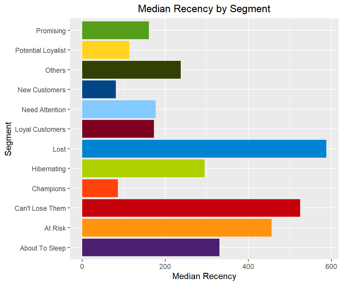
Median Frequency
rfm_plot_median_frequency(segments)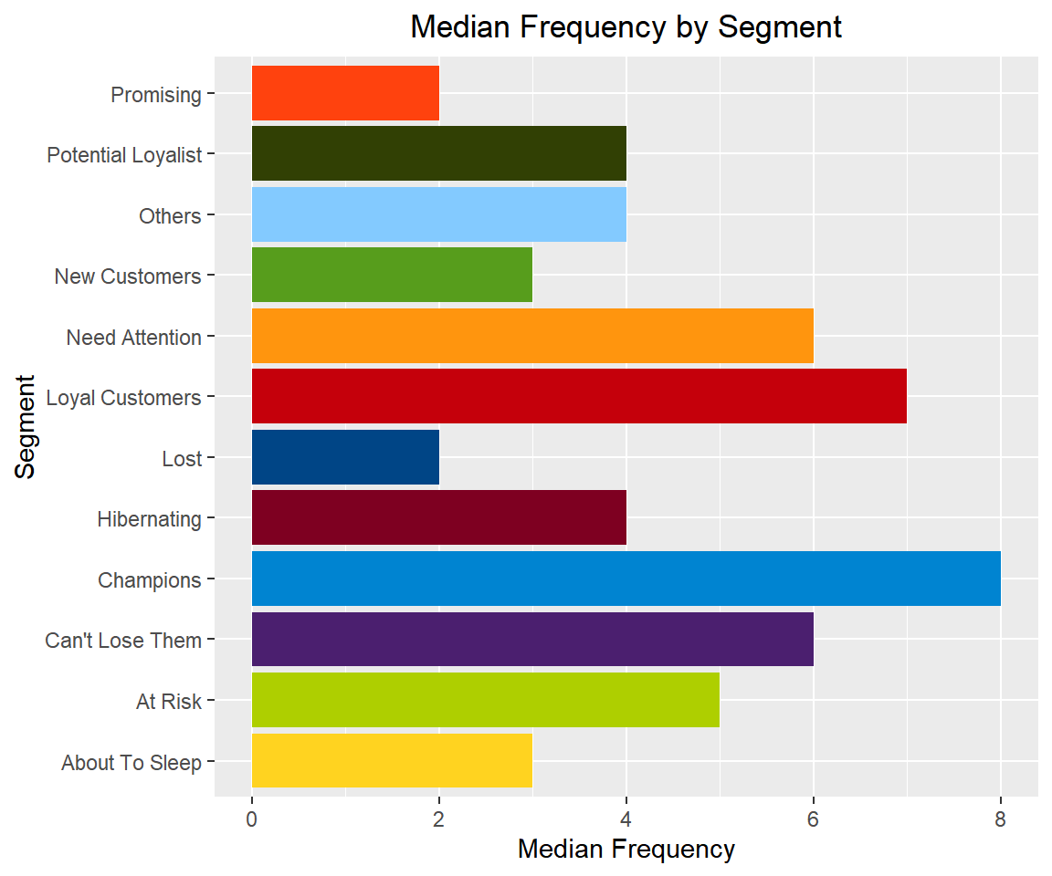
Median Monetary Value
rfm_plot_median_monetary(segments)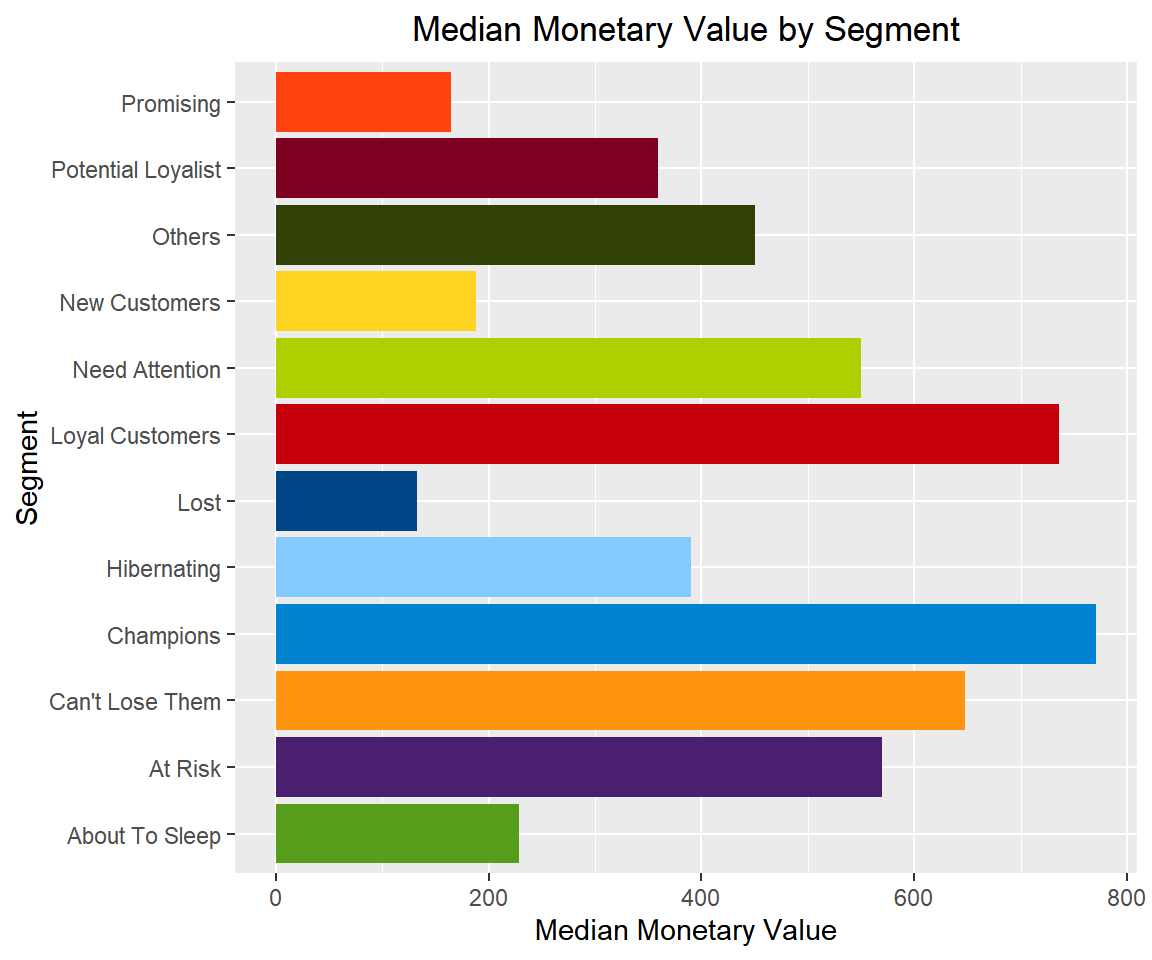
Heat Map
The heat map shows the average monetary value for different categories of recency and frequency scores. Higher scores of frequency and recency are characterized by higher average monetary value as indicated by the darker areas in the heatmap.
rfm_heatmap(rfm_result)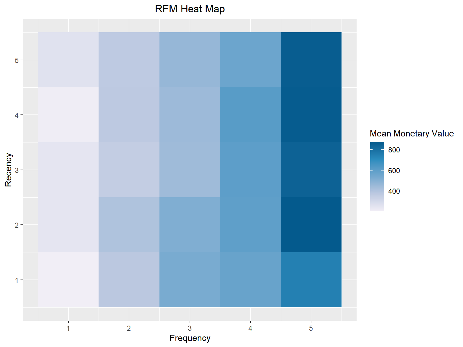
Bar Chart
Use rfm_bar_chart() to generate the distribution of monetary scores for the
different combinations of frequency and recency scores.
rfm_bar_chart(rfm_result)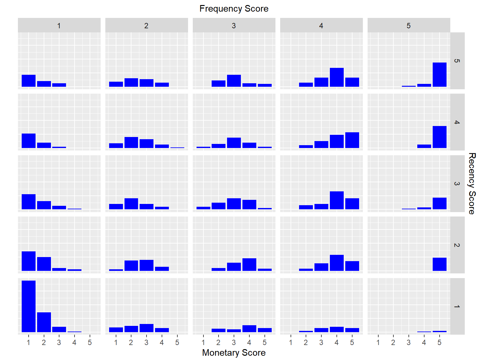
Histogram
Use rfm_histograms() to examine the relative distribution of
- monetary value (total revenue generated by each customer)
- recency days (days since the most recent visit for each customer)
- frequency (transaction count for each customer)
rfm_histograms(rfm_result)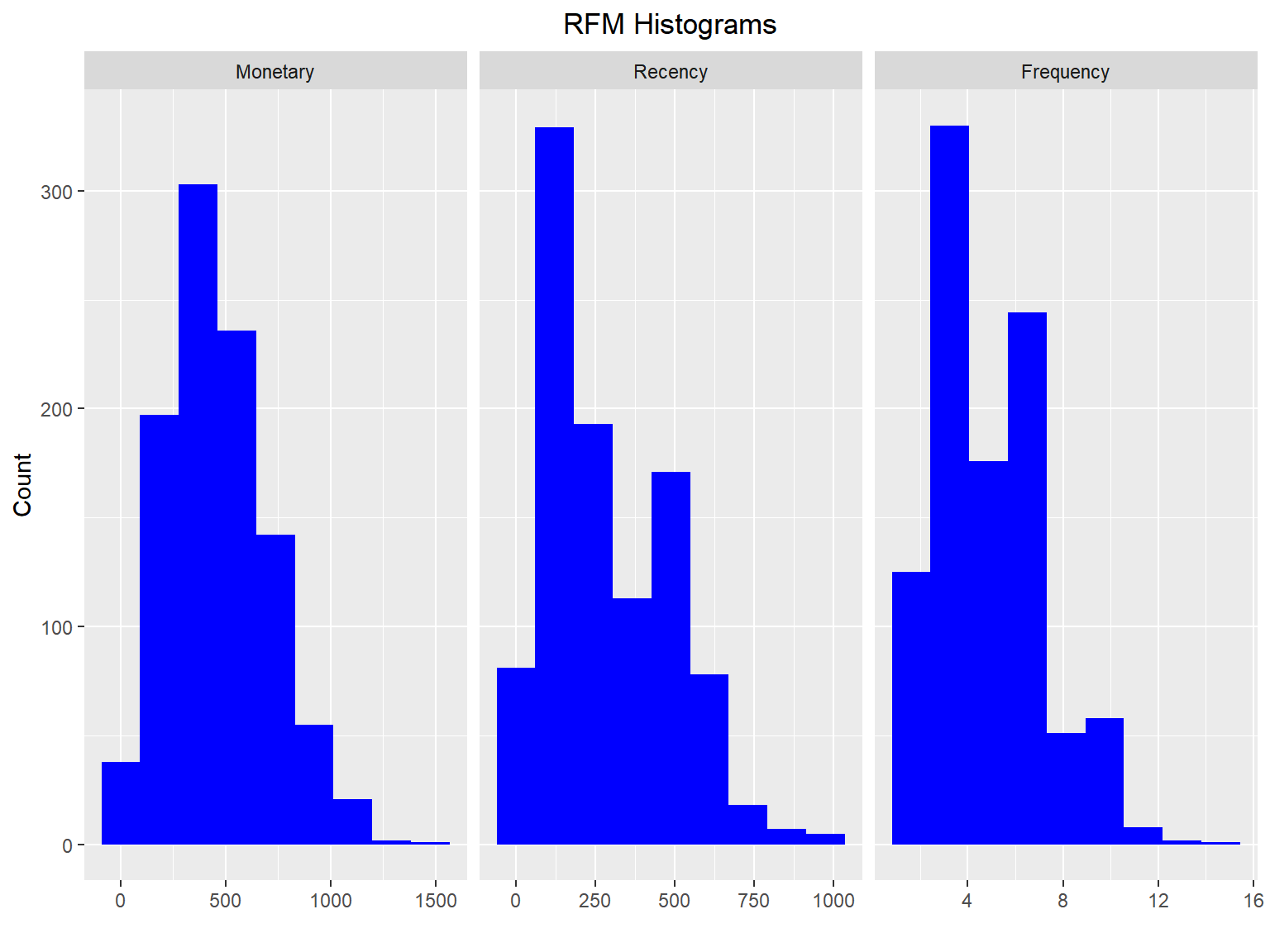
Customers by Orders
Visualize the distribution of customers across orders.
rfm_order_dist(rfm_result)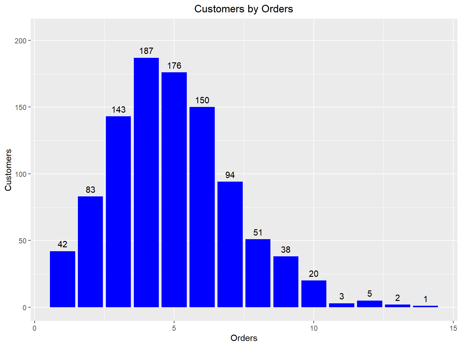
Scatter Plots
The best customers are those who:
- bought most recently
- most often
- and spend the most
Now let us examine the relationship between the above.
Recency vs Monetary Value
Customers who visited more recently generated more revenue compared to those who visited in the distant past. The customers who visited in the recent past are more likely to return compared to those who visited long time ago as most of those would be lost customers. As such, higher revenue would be associated with most recent visits.
rfm_rm_plot(rfm_result)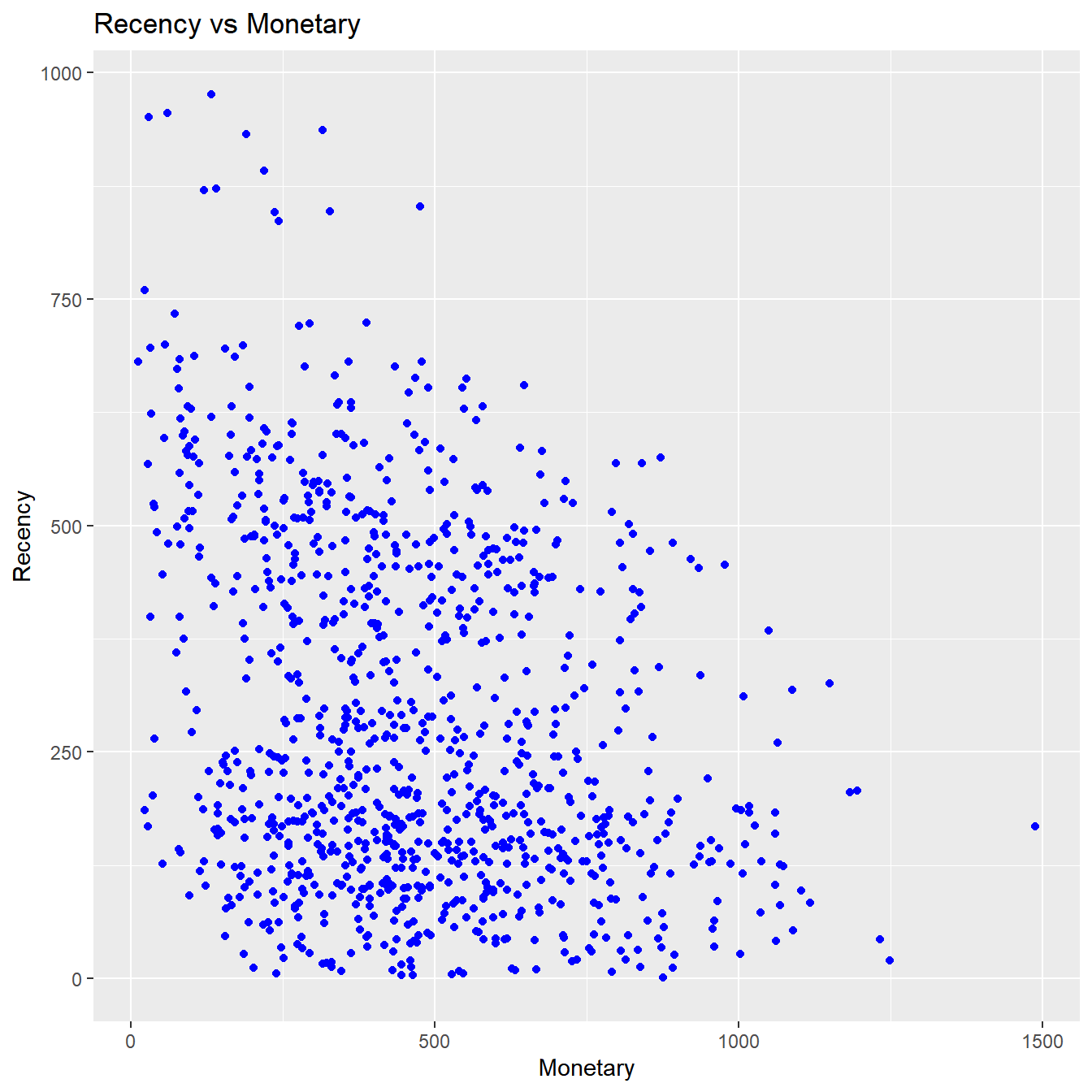
Frequency vs Monetary Value
As the frequency of visits increases, the revenue generated also increases. Customers who visit more frquently are your champion customers, loyal customers or potential loyalists and they drive higher revenue.
rfm_fm_plot(rfm_result)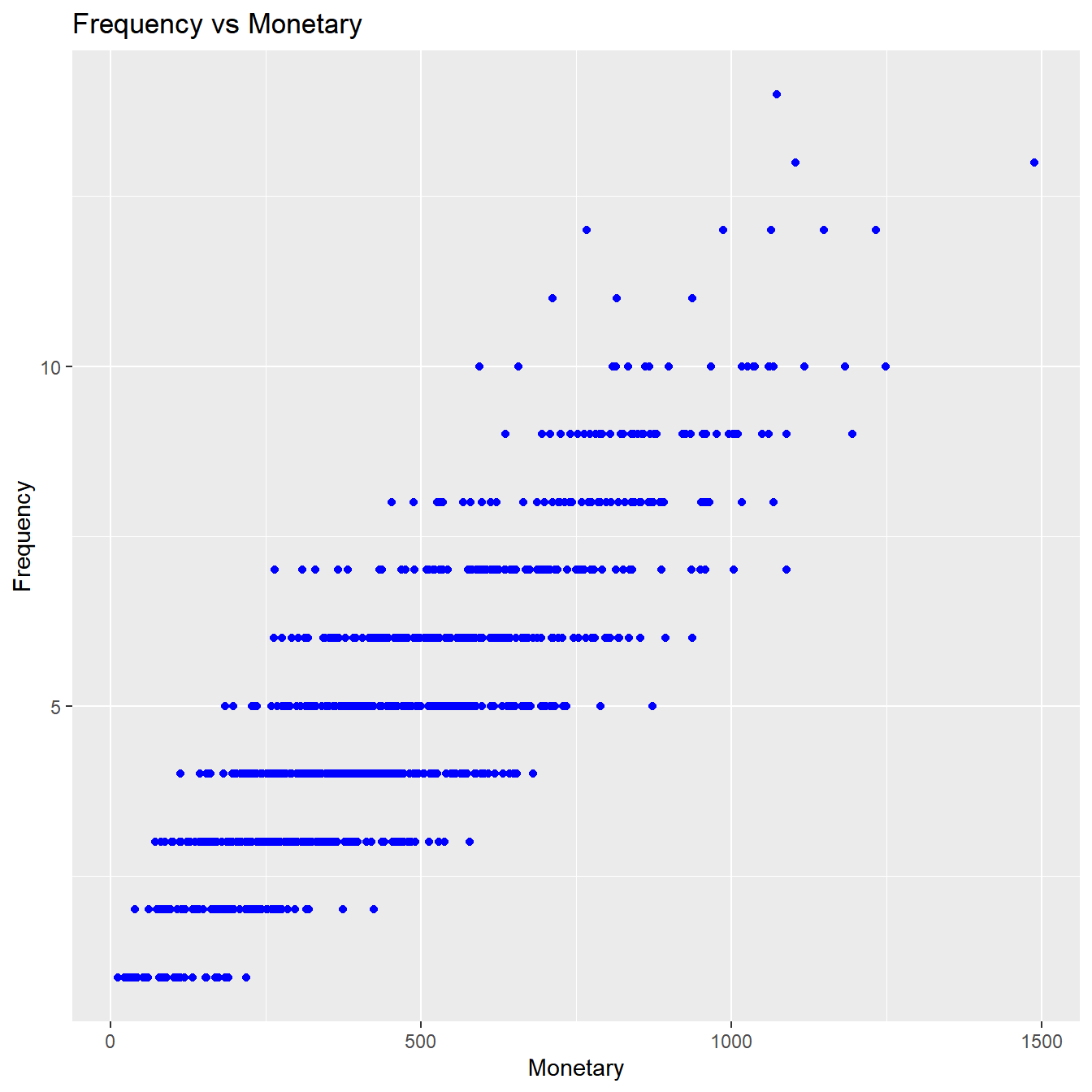
Recency vs Frequency
Customers with low frequency visited in the distant past while those with high frequency have visited in the recent past. Again, the customers who visited in the recent past are more likely to return compared to those who visited long time ago. As such, higher frequency would be associated with the most recent visits.
rfm_rf_plot(rfm_result)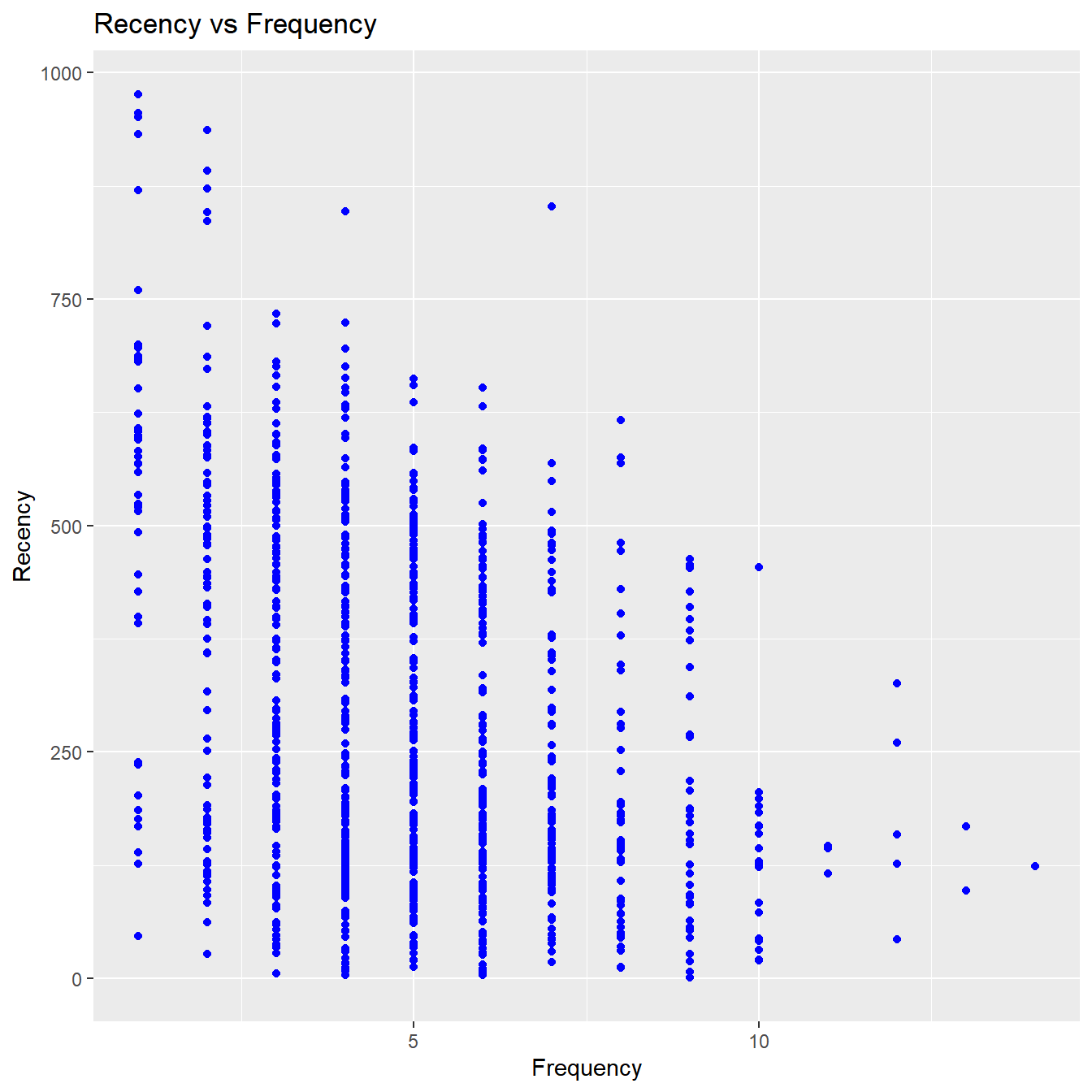
Your Turn…
if you look at the distribution of segments, around 13% of the customers are in the
Otherssegment For segmentation to be effective and optimal, theOtherssegment should be eliminated or should have few customers only. Redefine the segments and try to reduce the number of customers in theOtherssegment.we have defined 11 segments. Try to combine some of the existing segments and bring down the total segments to around 6 or 8.
the RFM score we generated uses score between 1 and 5. Try to create segments by using a score between 1 and 3 i.e. the lowest RFM should be 111 and the highest should be 333 instead of 555.
reverse the scores i.e. so far we have assigned a score of 5 to customers who visited recently, frequently and had higher transaction amount and 1 to customers who visited way back, rarely and have low transaction amount. Reverse this score pattern and create the segments.
Learning More
The rfm website includes comprehensive documentation on using the package, including the following articles that cover various aspects of using rfm:
RFM Customer Level Data - shows you how to handle customer level data.
RFM Transaction Level Data - shows you how to handle transaction level data.
Feedback
If you see mistakes or want to suggest changes, please create an issue on the source repository or reach out to us at support@rsquaredacademy.com.